

Chapter 1: Introduction to Timeseries#
by Julien Emile-Geay, University of Southern California
Background#
Recall that a timeseries \(X(t)\) is an ordered data sequence, either continuous or discrete. On a computer, everything is discretized, so regardless of the original process, what we have is a discrete sequence \(X_1, \cdots, X_n\), with each \(X_i\) corresponding to times \(t_i\) in \(t_1, \cdots, t_n\).
In timeseries analysis, it is common to consider \(X(t)\) as the sum of one or more oscillatory, stationary components (or ``signals’’); a trend \(q(t)\), and noise \(\varepsilon_t\). The oscillatory components are often the reason we’re doing the analysis in the first place – it will tell us how big they are and what their frequency is.
Whether or not those oscillatory components are present, a trend is often present as well. In today’s world the word “trend” is so overused that it has lost all meaning. Here, it will refer to a slowly-evolving, non-stationary component that dominates the behavior of the timeseries. For instance: a linear increase or decrease; a sinusoidal component so slow that its period is not resolved by the dataset; a nonlinear trend like the exponential increase of the Keeling curve (see below).
As for noise, it clearly involves a subjective definition. Under this name we usually subsume any variable component in which we are not interested. Some of this noise may be composed of actual measurement errors (what you would think of as noise, strictly speaking), but some of it could be what another analyst would call “signal””. If you study climate, daily fluctuations are noise; if you study weather, they are your signal. One commonly says that one analyst’s signal is another analyst’s noise. This noise is often modeled as a Normal random process with zero mean, \(\varepsilon \sim \mathcal{N}(0,\sigma^2)\) (aka “Gaussian white noise”) .
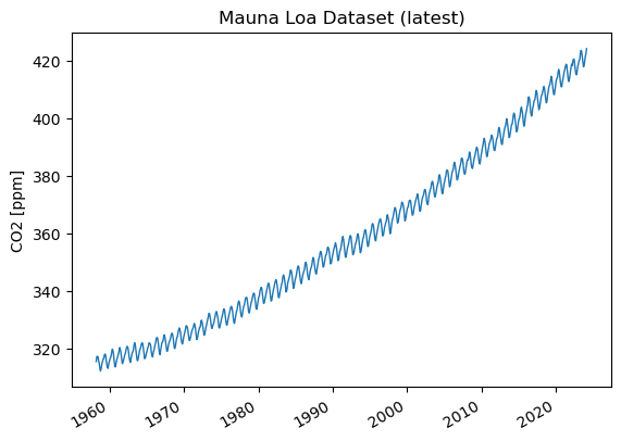
To see these concepts in action, let us consider the iconic Keeling curve from the Mauna Loa Observatory \(CO_2\) measurements. The data are available here. In addition to the usual scientific Python stack, we will be using pandas and statsmodels. Let us load these packages:
from matplotlib import pyplot as plt
import numpy as np
import pandas as pd
import warnings
warnings.filterwarnings('ignore')
Data Wrangling#
We use pandas to load the data, which are in csv. Pandas can load directly over the network, so all we need to give it is a URL of the file (here, https://scrippsco2.ucsd.edu/assets/data/atmospheric/stations/in_situ_co2/monthly/monthly_in_situ_co2_mlo.csv). Let’s try it:
url = 'https://scrippsco2.ucsd.edu/assets/data/atmospheric/stations/in_situ_co2/monthly/monthly_in_situ_co2_mlo.csv'
df = pd.read_csv(url)
df.head() # this will show the first few rows of the dataset
---------------------------------------------------------------------------
ParserError                               Traceback (most recent call last)
Cell In[2], line 2
      1 url = 'https://scrippsco2.ucsd.edu/assets/data/atmospheric/stations/in_situ_co2/monthly/monthly_in_situ_co2_mlo.csv'
----> 2 df = pd.read_csv(url)
      3 df.head()

File ~/opt/miniconda3/envs/pyleo/lib/python3.11/site-packages/pandas/io/parsers/readers.py:948, in read_csv(filepath_or_buffer, sep, delimiter, header, names, index_col, usecols, dtype, engine, converters, true_values, false_values, skipinitialspace, skiprows, skipfooter, nrows, na_values, keep_default_na, na_filter, verbose, skip_blank_lines, parse_dates, infer_datetime_format, keep_date_col, date_parser, date_format, dayfirst, cache_dates, iterator, chunksize, compression, thousands, decimal, lineterminator, quotechar, quoting, doublequote, escapechar, comment, encoding, encoding_errors, dialect, on_bad_lines, delim_whitespace, low_memory, memory_map, float_precision, storage_options, dtype_backend)
    935 kwds_defaults = _refine_defaults_read(
    936     dialect,
    937     delimiter,
   (...)
    944     dtype_backend=dtype_backend,
    945 )
    946 kwds.update(kwds_defaults)
--> 948 return _read(filepath_or_buffer, kwds)

File ~/opt/miniconda3/envs/pyleo/lib/python3.11/site-packages/pandas/io/parsers/readers.py:617, in _read(filepath_or_buffer, kwds)
    614     return parser
    616 with parser:
--> 617     return parser.read(nrows)

File ~/opt/miniconda3/envs/pyleo/lib/python3.11/site-packages/pandas/io/parsers/readers.py:1748, in TextFileReader.read(self, nrows)
   1741 nrows = validate_integer("nrows", nrows)
   1742 try:
   1743     # error: "ParserBase" has no attribute "read"
   1744     (
   1745         index,
   1746         columns,
   1747         col_dict,
-> 1748     ) = self._engine.read(  # type: ignore[attr-defined]
   1749         nrows
   1750     )
   1751 except Exception:
   1752     self.close()

File ~/opt/miniconda3/envs/pyleo/lib/python3.11/site-packages/pandas/io/parsers/c_parser_wrapper.py:234, in CParserWrapper.read(self, nrows)
    232 try:
    233     if self.low_memory:
--> 234         chunks = self._reader.read_low_memory(nrows)
    235         # destructive to chunks
    236         data = _concatenate_chunks(chunks)

File parsers.pyx:843, in pandas._libs.parsers.TextReader.read_low_memory()

File parsers.pyx:904, in pandas._libs.parsers.TextReader._read_rows()

File parsers.pyx:879, in pandas._libs.parsers.TextReader._tokenize_rows()

File parsers.pyx:890, in pandas._libs.parsers.TextReader._check_tokenize_status()

File parsers.pyx:2058, in pandas._libs.parsers.raise_parser_error()

ParserError: Error tokenizing data. C error: Expected 1 fields in line 35, saw 4
Question#
Q: What went wrong? To debug, you’ll have to download the file and look at it (do it). What do you see that a machine might have problems with?
Hint: https://www.askpython.com/python-modules/pandas/pandas-read-csv-with-headers
A: This csv file has a long header. pandas needs to be told how many lines to skip.
Another issue is that the name of the columns for the dataset span two rows, which pandas won’t be able to deal with on its own. So we need to give it 2 pieces of information:
How long the header is
What the column names are (which we can lift from the header manually)
We do this by passing two extra arguments to read_csv():
cols = ['Yr','Mn','XLDate','Date','CO2','seasonally adjusted','fit','seasonally adjusted fit','CO2 filled',	'seasonally adjusted filled','Sta']
df = pd.read_csv(url,header=64, names=cols) # read in the data
df.head() # display the top
| Yr | Mn | XLDate | Date | CO2 | seasonally adjusted | fit | seasonally adjusted fit | CO2 filled | seasonally adjusted filled | Sta | |
|---|---|---|---|---|---|---|---|---|---|---|---|
| 0 | 1958 | 2 | 21231 | 1958.1260 | -99.99 | -99.99 | -99.99 | -99.99 | -99.99 | -99.99 | MLO |
| 1 | 1958 | 3 | 21259 | 1958.2027 | 315.71 | 314.44 | 316.20 | 314.91 | 315.71 | 314.44 | MLO |
| 2 | 1958 | 4 | 21290 | 1958.2877 | 317.45 | 315.16 | 317.30 | 314.99 | 317.45 | 315.16 | MLO |
| 3 | 1958 | 5 | 21320 | 1958.3699 | 317.51 | 314.69 | 317.89 | 315.07 | 317.51 | 314.69 | MLO |
| 4 | 1958 | 6 | 21351 | 1958.4548 | -99.99 | -99.99 | 317.27 | 315.15 | 317.27 | 315.15 | MLO |
By default, pandas indexed the rows by their number (starting at 0 as it’s Python). Let’s extract the actual dates, convert them to a usable format, and re-index the dataframe:
date = pd.to_datetime(df['XLDate'], unit='D', origin='1899-12-30') # convert from Excel's weird standard to something human-readable
date.name = None
df.index=date
df.head()
| Yr | Mn | XLDate | Date | CO2 | seasonally adjusted | fit | seasonally adjusted fit | CO2 filled | seasonally adjusted filled | Sta | |
|---|---|---|---|---|---|---|---|---|---|---|---|
| 1958-02-15 | 1958 | 2 | 21231 | 1958.1260 | -99.99 | -99.99 | -99.99 | -99.99 | -99.99 | -99.99 | MLO |
| 1958-03-15 | 1958 | 3 | 21259 | 1958.2027 | 315.71 | 314.44 | 316.20 | 314.91 | 315.71 | 314.44 | MLO |
| 1958-04-15 | 1958 | 4 | 21290 | 1958.2877 | 317.45 | 315.16 | 317.30 | 314.99 | 317.45 | 315.16 | MLO |
| 1958-05-15 | 1958 | 5 | 21320 | 1958.3699 | 317.51 | 314.69 | 317.89 | 315.07 | 317.51 | 314.69 | MLO |
| 1958-06-15 | 1958 | 6 | 21351 | 1958.4548 | -99.99 | -99.99 | 317.27 | 315.15 | 317.27 | 315.15 | MLO |
Next, let’s extract the column that we want to play with and make a new data frame out of it:
co2 = df[['Date','CO2 filled']]
co2.rename(columns={'Date': 'Year', 'CO2 filled': 'CO2'},inplace=True) # rename columns for clarity
co2.head()
| Year | CO2 | |
|---|---|---|
| 1958-02-15 | 1958.1260 | -99.99 |
| 1958-03-15 | 1958.2027 | 315.71 |
| 1958-04-15 | 1958.2877 | 317.45 |
| 1958-05-15 | 1958.3699 | 317.51 |
| 1958-06-15 | 1958.4548 | 317.27 |
One last thing: the first and last value are missing, and they are encoded as -99, which is rather annoying (but unfortunately common; NaN would be a much less disruptive choice), so let’s restrict our analysis to a safe, 66y interval:
co2 = co2.loc['1958-03-15':'2024-02-15']
Now we can sit back and admire our work.
Question#
Q: plot CO2 as a function of time
Hint: use pandas’s plot function.
A:
co2['CO2'].plot(linewidth=1,ylabel='CO2 [ppm]',title="Mauna Loa Dataset (latest)")
<Axes: title={'center': 'Mauna Loa Dataset (latest)'}, ylabel='CO2 [ppm]'>
Now we can sit back and admire our work.
Question#
Q: plot CO2 as a function of time
Hint: use pandas’s plot function.
A:
2. Trend Extraction#
2.1 Linear trend model#
The most obvious thing to do is to see if a linear trend might fit the data. In this case it’s likely to be a poor approximation, as the previous plot should make obvious. However, it will be an instructive benchmarks for the finer modeling choices we’ll subsequently make.
Let’s first load the statsmodels API (=Application Programming Interface) to use its packages. What is happening under the hood is a simple linear regression, which you don’t need to know much about at this stage. Specifically, we will use the OLS method. which relates a predictand \(y\) to a matrix of predictors \(X\), called the design matrix.
t = co2['Year']
y = co2['CO2']
X = np.vander(t, 2) # set up design matrix with 1, t as predictors

import statsmodels.api as sm
lin_mdl = sm.OLS(y, X).fit() # fit the OLS model to the observations
Let’s pause and contemplate this, for a moment.
First, we set up the design matrix X as a Vandermonde matrix; there is nothing particularly profound here; it is just a nice way to set this up in one function call. Second, we fit the model and that just involved importing a module and calling a fit() function. You have NO IDEA how lucky you are to have grown up in an age where fitting statistical models is that easy. Just like democracy, this is someting that has cost the blood, sweat and tears of countless generations before you, so you had better be grateful!
But there’s more. stasmodels is an example of object-oriented programming. It means that every model object created by this code enjoys a wide array of properties and utilities.
The first is a stunningly gorgeous summary of the model fit:
print(lin_mdl.summary())
                            OLS Regression Results
==============================================================================
Dep. Variable:                    CO2   R-squared:                       0.976
Model:                            OLS   Adj. R-squared:                  0.976
Method:                 Least Squares   F-statistic:                 3.162e+04
Date:                Tue, 21 May 2024   Prob (F-statistic):               0.00
Time:                        15:37:39   Log-Likelihood:                -2382.0
No. Observations:                 792   AIC:                             4768.
Df Residuals:                     790   BIC:                             4777.
Df Model:                           1
Covariance Type:            nonrobust
==============================================================================
                 coef    std err          t      P>|t|      [0.025      0.975]
------------------------------------------------------------------------------
x1             1.6262      0.009    177.832      0.000       1.608       1.644
const      -2879.4377     18.210   -158.127      0.000   -2915.183   -2843.693
==============================================================================
Omnibus:                       46.565   Durbin-Watson:                   0.066
Prob(Omnibus):                  0.000   Jarque-Bera (JB):               45.317
Skew:                           0.535   Prob(JB):                     1.44e-10
Kurtosis:                       2.524   Cond. No.                     2.08e+05
==============================================================================

Notes:
[1] Standard Errors assume that the covariance matrix of the errors is correctly specified.
[2] The condition number is large, 2.08e+05. This might indicate that there are
strong multicollinearity or other numerical problems.
For more information about what each term means, see this post
What information can you glean from this summary? What features would you check for in a visual inspection?
[ANSWER HERE]
Let us look at the plot, shall we? How well does the time variable predict \(CO_2\)?
Next, we can use the predict() method to predict CO2 given the design matrix (1, \(t\))
yhat = lin_mdl.predict(X)
plt.plot(t, y, label="MLO data",linewidth=1)
plt.plot(t, yhat, label=r"$CO_2 = \beta_0 + \beta_1 t$", color='black', linewidth='2')
plt.ylabel(r"$CO_2$")
plt.xlabel("Date")
plt.legend()
<matplotlib.legend.Legend at 0x176952b30>
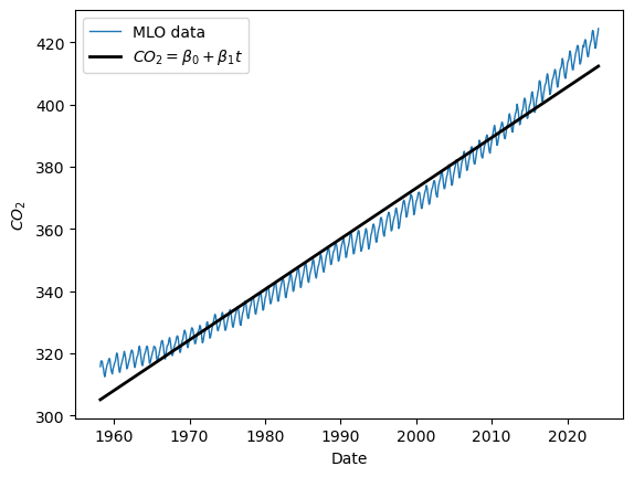
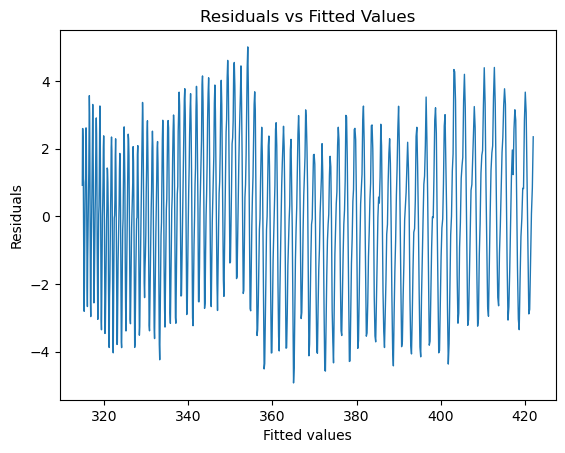
We see that the line captures the first order behavior of the series, but that leaves a lot to be desired. To zoom in, we can look at the residuals (original values - fitted values) as a function of fitted values:
fig, ax = plt.subplots()
ax.plot(lin_mdl.fittedvalues,lin_mdl.resid,linewidth=1)
ax.set_title('Residuals vs Fitted Values')
ax.set_xlabel('Fitted values')
ax.set_ylabel('Residuals')
Text(0, 0.5, 'Residuals')
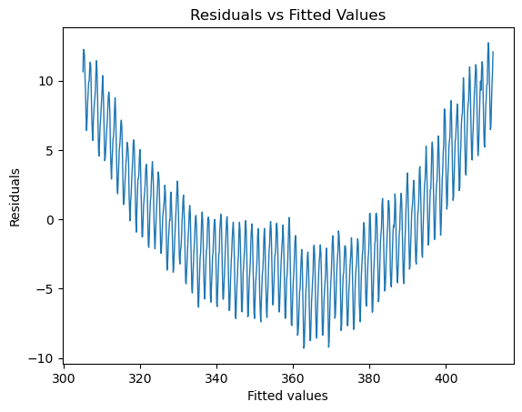
To be quantitative, we can look at the Root Mean Squared Error of these residuals:
print('RMSE = ' + '{:4.4f}'.format(np.sqrt(lin_mdl.mse_resid)) + ' ppm')
RMSE = 4.9033 ppm
This means that this linear trend is, on average, about 5ppm away from the measurements. Can we do better?
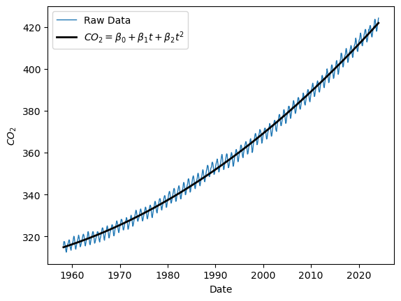
2.2. Quadratic fit#
The second thing one might do is to add a quadratic term. Again, the Vandermonde matrix makes this very easy:
X = np.vander(t, 3) # set up design matrix with 1, t, and t^2 as predictors
quad_mdl = sm.OLS(y, X).fit()
print(quad_mdl.summary())
# plot predicted values
yhat = quad_mdl.predict(X)
plt.plot(t, y, label="Raw Data",linewidth=1)
plt.plot(t, yhat, label=r"$CO_2 = \beta_0 + \beta_1 t + \beta_2 t^2$", color='black', linewidth='2')
plt.ylabel(r"$CO_2$")
plt.xlabel("Date")
plt.legend()
                            OLS Regression Results
==============================================================================
Dep. Variable:                    CO2   R-squared:                       0.995
Model:                            OLS   Adj. R-squared:                  0.995
Method:                 Least Squares   F-statistic:                 7.812e+04
Date:                Tue, 21 May 2024   Prob (F-statistic):               0.00
Time:                        15:38:01   Log-Likelihood:                -1756.7
No. Observations:                 792   AIC:                             3519.
Df Residuals:                     789   BIC:                             3533.
Df Model:                           2
Covariance Type:            nonrobust
==============================================================================
                 coef    std err          t      P>|t|      [0.025      0.975]
------------------------------------------------------------------------------
x1             0.0134      0.000     55.121      0.000       0.013       0.014
x2           -51.8912      0.971    -53.446      0.000     -53.797     -49.985
const        5.04e+04    966.564     52.140      0.000    4.85e+04    5.23e+04
==============================================================================
Omnibus:                      118.499   Durbin-Watson:                   0.317
Prob(Omnibus):                  0.000   Jarque-Bera (JB):               30.044
Skew:                          -0.108   Prob(JB):                     2.99e-07
Kurtosis:                       2.071   Cond. No.                     4.84e+10
==============================================================================

Notes:
[1] Standard Errors assume that the covariance matrix of the errors is correctly specified.
[2] The condition number is large, 4.84e+10. This might indicate that there are
strong multicollinearity or other numerical problems.
<matplotlib.legend.Legend at 0x1769e2ef0>
fig, ax = plt.subplots()
ax.plot(quad_mdl.fittedvalues,quad_mdl.resid,linewidth=1)
ax.set_title('Residuals vs Fitted Values')
ax.set_xlabel('Fitted values')
ax.set_ylabel('Residuals')
print('RMSE = ' + '{:4.4f}'.format(np.sqrt(quad_mdl.mse_resid)) + ' ppm')
RMSE = 2.2277 ppm
Question 3 Does this improve the fit? By how much have we shrunk the RMSE of residuals?
Comment in detail on how the addition of a quadratic term has changed plots a, b c and d. What issues have been solved? What issues remain?
[ANSWERS HERE]
3. Adding Periodic components#
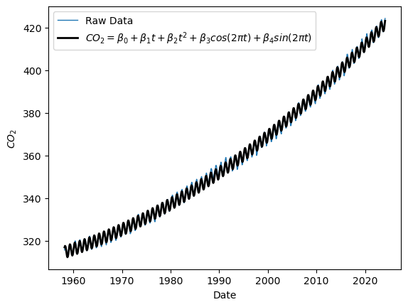
It should be obvious from the simple visual inspection of the original series that there is a strong periodic component we are not currently capturing. It turns out to the a simple seasonal cycle: in spring/summer, the growth of terrestrial biomass sequesters CO2 away from the atmosphere, so the atmospheric CO2 concentrations goes down; the reverse happens in the Fall/Winter, where the fallen leaves are degraded and their organic carbon returned to mineral (CO2) form via respiration.
Let us thus define harmonic waves (sines and cosines) with a period of 1 year and add them to the design matrix.
H = np.column_stack((np.cos(2*np.pi*t),np.sin(2*np.pi*t)))
Xh = np.concatenate((np.vander(t, 3),H),axis=1)
seas_mdl = sm.OLS(y, Xh).fit()
print(seas_mdl.summary())
# plot predicted values
yhat = seas_mdl.predict(Xh)
plt.plot(t, y, label="Raw Data",linewidth=1)
plt.plot(t, yhat, label=r"$CO_2 = \beta_0 + \beta_1 t + \beta_2 t^2 + \beta_3 cos(2\pi t) + \beta_4 sin(2\pi t)  $", color='black', linewidth='2')
plt.ylabel(r"$CO_2$")
plt.xlabel("Date")
plt.legend()
                            OLS Regression Results
==============================================================================
Dep. Variable:                    CO2   R-squared:                       0.999
Model:                            OLS   Adj. R-squared:                  0.999
Method:                 Least Squares   F-statistic:                 2.213e+05
Date:                Tue, 21 May 2024   Prob (F-statistic):               0.00
Time:                        15:38:15   Log-Likelihood:                -1070.5
No. Observations:                 792   AIC:                             2151.
Df Residuals:                     787   BIC:                             2174.
Df Model:                           4
Covariance Type:            nonrobust
==============================================================================
                 coef    std err          t      P>|t|      [0.025      0.975]
------------------------------------------------------------------------------
x1             0.0134      0.000    130.916      0.000       0.013       0.014
x2           -51.8860      0.409   -126.934      0.000     -52.688     -51.084
const       5.039e+04    406.930    123.831      0.000    4.96e+04    5.12e+04
x3            -1.0027      0.047    -21.233      0.000      -1.095      -0.910
x4             2.6689      0.047     56.733      0.000       2.577       2.761
==============================================================================
Omnibus:                        8.817   Durbin-Watson:                   0.529
Prob(Omnibus):                  0.012   Jarque-Bera (JB):                6.328
Skew:                           0.090   Prob(JB):                       0.0423
Kurtosis:                       2.600   Cond. No.                     4.84e+10
==============================================================================

Notes:
[1] Standard Errors assume that the covariance matrix of the errors is correctly specified.
[2] The condition number is large, 4.84e+10. This might indicate that there are
strong multicollinearity or other numerical problems.
<matplotlib.legend.Legend at 0x176bf2fe0>
fig, ax = plt.subplots()
ax.plot(seas_mdl.fittedvalues,seas_mdl.resid,linewidth=1, alpha = 0.6)
ax.set_title('Residuals vs Fitted Values')
ax.set_xlabel('Fitted values')
ax.set_ylabel('Residuals')
print('RMSE = ' + '{:4.4f}'.format(np.sqrt(seas_mdl.mse_resid)) + ' ppm')
RMSE = 0.9379 ppm
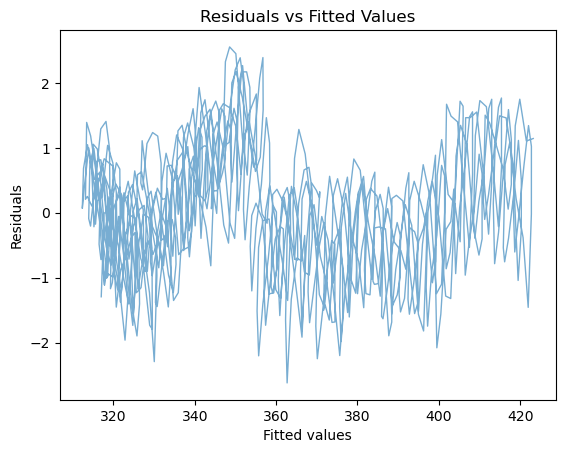
Question 4
This should look better. Does it? By how much have we shrunk the RMSE of residuals?
print('{:4.4f}'.format(100*(1-np.sqrt(seas_mdl.mse_resid/lin_mdl.mse_resid))))
80.8727
Answer: over 80% improvement!
Seasonal-Trend decomposition using LOESS (STL)#
As it turns out, statsmodels already contains much more sophisticated tools to do this sort of work. Witness STL decomposition in action:
from statsmodels.tsa.seasonal import STL
co2_s = pd.Series(
    co2['CO2'].values, index=pd.date_range("3-15-1958", periods=len(co2), freq="M"), name="CO2"
)
stl = STL(co2_s, seasonal=13)
stl_res = stl.fit()
fig = stl_res.plot()
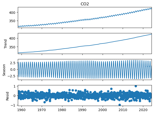
rmse = np.sqrt(np.square(stl_res._resid.values).mean())
print('RMSE = ' + '{:4.4f}'.format(rmse) + ' ppm')
RMSE = 0.2215 ppm
As we can see, this decomposition got us much, much closer to the observations, with an RMSE of just 0.22 ppm. This is because the seasonal cycle is allowed to fluctuate in amplitude, and the trend is also more general than a quadratic. However, this is more of a black box.
4. Forecasting#
Let us return to our parametric model of atmospheric \(CO_2\) (quadractic trend + seasonal harmonics), which we may use to forecast future observations. Let’s extend our time axis to 2050 and see what \(CO_2\) may look like then if we don’t curb emissions or fail to remove it from the atmosphere:
tn = t.to_numpy()
dt = np.diff(tn)[0]
tf = np.arange(max(tn)+dt,2050,dt)
tp = np.concatenate((tn,tf))
nf = len(tf) #number of future values to forecast
Hp = np.column_stack((np.cos(2*np.pi*tp),np.sin(2*np.pi*tp)))
Xp = np.concatenate((np.vander(tp, 3),Hp),axis=1)

yh = seas_mdl.predict(Xp)
plt.plot(t, y,'k.',alpha=0.5, label="Raw Data")
plt.plot(tp, yh, label=r"$CO_2 = \beta_0 + \beta_1 t + \beta_2 t^2 + \beta_3 cos(2\pi t) + \beta_4 sin(2\pi t)  $", linewidth='2')
plt.ylabel(r"$CO_2$")
plt.xlabel("Date")
plt.legend()
<matplotlib.legend.Legend at 0x176b4a8f0>
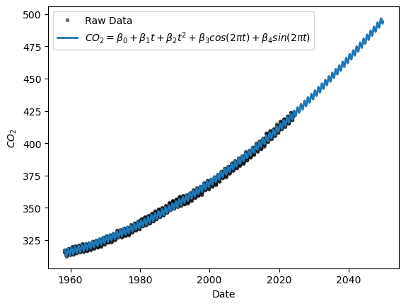
From this, one can estimate. e.g. the time of first crossing 450 ppm, for instance.
Of course, those predictions are only as good as the data that went into them, and the assumptions that the same processes will continue to operate at the same rate. Note that there are much more sophisticated methods for timeseries forecasting basd on machine learning, e.g. tsfresh. Another option that would likely work here is using seasonal ARIMA models, as done here.