pyODV#
Overview#
Ocean Data Viewer is a nifty piece of software for visualizing gridded data like the World Ocean Atlas. This notebook provides tips about how to make similar plots as part of a Python based workflow.
Imports#
%load_ext autoreload
%autoreload 2

import numpy as np
import xarray as xr
import os
import pandas as pd
import seaborn as sns
from pathlib import Path

import matplotlib.pyplot as plt
import matplotlib as mpl
from matplotlib import cm
import matplotlib.gridspec as gridspec
from matplotlib.ticker import FormatStrFormatter
from mpl_toolkits.axes_grid1.inset_locator import inset_axes

import cartopy
import cartopy.crs as ccrs
import cartopy.feature as cfeature
import cartopy.util as cutil
import sys
module_path = str(Path(os.getcwd()).parent.parent/'support_functions')
if module_path not in sys.path:
    sys.path.append(module_path)

import data_processing as dp
import plotting_helpers as ph
lat_u = r'$^{\circ}$N'
lon_u = r'$^{\circ}$E'
depth_u = 'm'
time_u = 'ky BP'
eNd_label = r'$\varepsilon$Nd'

surface_title = 'depth={} '+depth_u+ ', time={} '+time_u
Load Data#
To run this notebook, you’ll need to point it to relevant data files. This notebook assumes files in which TLAT and TLONG are arrays of latitude and longitude values, and that z_t is a depth vector.
import fsspec

url = 'https://g-f750ca.a78b8.36fe.data.globus.org/C-iTRACE/ctrace.decadal.SALT.zarr'
mapper = fsspec.get_mapper(url)
ds = xr.open_zarr(mapper)

variables = [
    'CISO_DIC_d13C','ND143','ND144',
]

for var in variables:
    url = 'https://g-f750ca.a78b8.36fe.data.globus.org/C-iTRACE/ctrace.decadal.{}.zarr'.format(var)
    mapper = fsspec.get_mapper(url)
    _ds = xr.open_zarr(mapper)
    ds = ds.merge(_ds)

ds
<xarray.Dataset>
Dimensions:        (time: 2200, z_t: 60, nlat: 116, nlon: 100, d2: 2)
Coordinates:
    TLAT           (nlat, nlon) float64 dask.array<chunksize=(116, 100), meta=np.ndarray>
    TLONG          (nlat, nlon) float64 dask.array<chunksize=(116, 100), meta=np.ndarray>
  * time           (time) float64 -22.0 -21.99 -21.98 ... -0.03 -0.02 -0.01
  * z_t            (z_t) float32 500.0 1.5e+03 2.5e+03 ... 5.125e+05 5.375e+05
Dimensions without coordinates: nlat, nlon, d2
Data variables:
    SALT           (time, z_t, nlat, nlon) float32 dask.array<chunksize=(275, 8, 15, 25), meta=np.ndarray>
    time_bound     (time, d2) float64 dask.array<chunksize=(2200, 2), meta=np.ndarray>
    CISO_DIC_d13C  (time, z_t, nlat, nlon) float32 dask.array<chunksize=(275, 8, 15, 25), meta=np.ndarray>
    ND143          (time, z_t, nlat, nlon) float32 dask.array<chunksize=(275, 8, 15, 25), meta=np.ndarray>
    ND144          (time, z_t, nlat, nlon) float32 dask.array<chunksize=(275, 8, 15, 25), meta=np.ndarray>
Attributes: (12/16)
    Conventions:                CF-1.0; http://www.cgd.ucar.edu/cms/eaton/net...
    NCO:                        netCDF Operators version 4.9.5 (Homepage = ht...
    calendar:                   All years have exactly  365 days.
    cell_methods:               cell_methods = time: mean ==> the variable va...
    contents:                   Diagnostic and Prognostic Variables
    conventions:                CF-1.0; http://www.cgd.ucar.edu/cms/eaton/net...
    ...                         ...
    revision:                    $Name: ccsm3_0_1_beta22 $
    source:                     POP, the NCAR/CSM Ocean Component
    start_time:                 This dataset was created on 2007-07-29 at 23:...
    tavg_sum:                   2592000.0
    tavg_sum_qflux:             2592000.0
title: b30.22_0kaDVTExtract a small slice to make things more manageable..
time_slice = slice(-8, -5)
iso_ds = ds.sel(dict(time=time_slice)).copy()
Calculate \(\varepsilon\)Nd, add it to our mega-dataset and drop Nd144 and Nd143.
def epsNd(Nd):
    (Nd143, Nd144) = Nd
    Nd_CHUR = 0.512638
    scaler = 1000
    return (np.divide(Nd143,Nd144)*1/Nd_CHUR-1)*10**4
epsNd_tmp = xr.apply_ufunc(epsNd, (iso_ds['ND143'],iso_ds['ND144']))
epsNd_tmp.name = 'eNd'
iso_ds['eNd'] = (('time', 'z_t', 'nlat', 'nlon'), epsNd_tmp.squeeze().data)
iso_ds = iso_ds.drop_vars(['ND143', 'ND144']).squeeze()
We’ll add epsNd to data_processing.py for future use, just like we did for convert_z_to_meters and between which each first appeared in the notebook about working with data on a model grid.
# convert depth from cm to m
iso_ds =dp.convert_z_to_meters(iso_ds)
iso_ds
<xarray.Dataset>
Dimensions:        (time: 301, z_t_m: 60, nlat: 116, nlon: 100, d2: 2)
Coordinates:
    TLAT           (nlat, nlon) float64 dask.array<chunksize=(116, 100), meta=np.ndarray>
    TLONG          (nlat, nlon) float64 dask.array<chunksize=(116, 100), meta=np.ndarray>
  * time           (time) float64 -8.0 -7.99 -7.98 -7.97 ... -5.02 -5.01 -5.0
    z_t            (z_t_m) float32 500.0 1.5e+03 2.5e+03 ... 5.125e+05 5.375e+05
  * z_t_m          (z_t_m) float32 5.0 15.0 25.0 ... 5.125e+03 5.375e+03
Dimensions without coordinates: nlat, nlon, d2
Data variables:
    SALT           (time, z_t_m, nlat, nlon) float32 dask.array<chunksize=(250, 8, 15, 25), meta=np.ndarray>
    time_bound     (time, d2) float64 dask.array<chunksize=(301, 2), meta=np.ndarray>
    CISO_DIC_d13C  (time, z_t_m, nlat, nlon) float32 dask.array<chunksize=(250, 8, 15, 25), meta=np.ndarray>
    eNd            (time, z_t_m, nlat, nlon) float32 dask.array<chunksize=(250, 8, 15, 25), meta=np.ndarray>
Attributes: (12/16)
    Conventions:                CF-1.0; http://www.cgd.ucar.edu/cms/eaton/net...
    NCO:                        netCDF Operators version 4.9.5 (Homepage = ht...
    calendar:                   All years have exactly  365 days.
    cell_methods:               cell_methods = time: mean ==> the variable va...
    contents:                   Diagnostic and Prognostic Variables
    conventions:                CF-1.0; http://www.cgd.ucar.edu/cms/eaton/net...
    ...                         ...
    revision:                    $Name: ccsm3_0_1_beta22 $
    source:                     POP, the NCAR/CSM Ocean Component
    start_time:                 This dataset was created on 2007-07-29 at 23:...
    tavg_sum:                   2592000.0
    tavg_sum_qflux:             2592000.0
title: b30.22_0kaDVTtime = 5.99
iso_snapshot_data = iso_ds.sel(time = -time, method='nearest')
# iso_snapshot_data = iso_snapshot_data.compute()
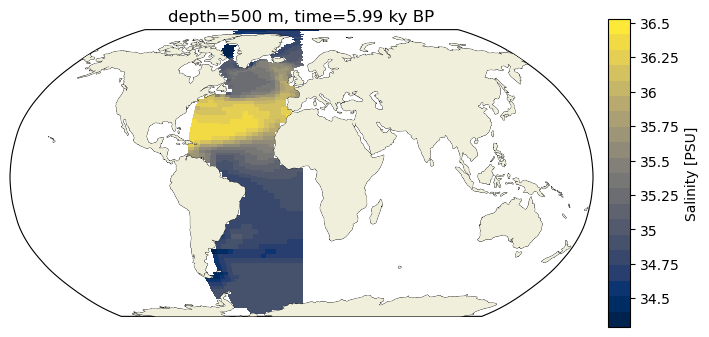
Surface: lon v. lat + color#
A surface plot looks the geographic distribution of some variable on a plane. Here, we’ll limit our area of interest to part of the Atlantic and pick a constant depth surface.
def between(ds, var, lims): _ds = ds.where((ds.coords[var]<max(lims)) & (ds.coords[var]>min(lims)), drop=True) return _ds
lonlims = [290, 360]
lon_ds = dp.between(iso_snapshot_data, 'TLONG', lonlims)
latlims = [-90, 90]
subarea_ds = dp.between(lon_ds, 'TLAT', latlims)
var = 'SALT'
colorbar_units='PSU'
depth = 500
iso_snapshot_data[var] =iso_snapshot_data[var].compute()#data.max()
surf_ds = subarea_ds.sel(z_t_m=depth, method='nearest')
c_snapshot_data_surf = surf_ds[var].squeeze()
c_snapshot_data_surf = c_snapshot_data_surf.compute()
Doesn’t hurt to take a quick look a the distribution of the data. Particularly given we will want to use a colorbar, it’s handy to check in on the range and density of values.
bins =surf_ds[var].compute().plot.hist()
bin_edges = bins[1]
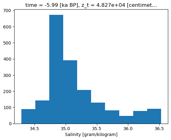
And now for the plot! There aren’t any raging outliers, so we’ll build our color mapping based on the full range of data.
# establish scale
max_lim = bin_edges[-1]#c_snapshot_data.max()
min_lim = bin_edges[0]#c_snapshot_data.min()
def make_scalar_mappable(lims, cmap, n=None):
ax_norm = mpl.colors.Normalize(vmin=min(lims), vmax=max(lims), clip=False)
if type(cmap)==list:
if n is None:
ax_cmap = mpl.colors.LinearSegmentedColormap.from_list(“MyCmapName”,cmap)
else:
ax_cmap = mpl.colors.LinearSegmentedColormap.from_list(“MyCmapName”,cmap, N=n)
else:
if n is None:
ax_cmap = plt.get_cmap(cmap)
else:
ax_cmap = plt.get_cmap(cmap, n)
ax_sm = cm.ScalarMappable(norm=ax_norm, cmap=ax_cmap)
return ax_sm
n_levels= 20
ax2_levels = np.around(np.linspace(min_lim, max_lim, n_levels), decimals=4)
# make scalar mappable
ax2_sm = ph.make_scalar_mappable([min_lim, max_lim],'cividis' , n_levels)
cf2_kwargs = {'cmap':ax2_sm.cmap,'levels':ax2_levels, 'norm' : ax2_sm.norm}
As discussed a bit in the notebook about the perils of model grids, there are a few ways to go about plotting spatial distributions. pcolormesh takes meshes of x and y values (in our case longitude and latitude) that underpin the data of interest (they do not need to fall on a regular rectangular grid) and interpolates between them.
fig = plt.figure(figsize=(8, 4))
# 1 row, 2 columns, .05 space between columns, 8:.3 ratio of left column to right column
gs = gridspec.GridSpec(1, 2, wspace=0.05, width_ratios=[8, .3])

# add subplot with specified map projection and coastlines (GeoAxes)
ax2 = fig.add_subplot(gs[0, 0], projection=ccrs.Robinson(central_longitude=0))

c_snapshot_data_surf.plot.pcolormesh(ax=ax2,
                                   transform=ccrs.PlateCarree(),
                                   x='TLONG', y='TLAT',
                                   levels=ax2_levels,
                                  cmap=cf2_kwargs['cmap'],
                                  norm=cf2_kwargs['norm'],
                                  add_colorbar=False);

ax2.coastlines(linewidth=.5)
ax2.add_feature(cfeature.LAND, zorder=14)

ax2_cb = fig.add_subplot(gs[0, 1])
cb2 = plt.colorbar(ax2_sm,cax=ax2_cb, orientation='vertical',label='{} [{}]'.format('Salinity',colorbar_units),
                   format=FormatStrFormatter('%g'))

ax2.set_title(surface_title.format(depth, time));
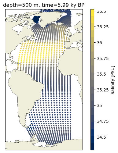
Alternatively, we can also just make a scatterplot, which has the advantage of making the point density explicity.
fig = plt.figure(figsize=(4, 6))
# 1 row, 2 columns, .05 space between columns, 8:.3 ratio of left column to right column
gs = gridspec.GridSpec(1, 2, wspace=0.05, width_ratios=[8, .3])

# add subplot with specified map projection and coastlines (GeoAxes)
ax2 = fig.add_subplot(gs[0, 0], projection=ccrs.Robinson(central_longitude=0))
ax2.add_feature(cfeature.COASTLINE, edgecolor='k',linewidth=.5)

ax2.scatter(c_snapshot_data_surf.TLONG,c_snapshot_data_surf.TLAT,c=c_snapshot_data_surf,
            transform=ccrs.PlateCarree(),
            cmap=cf2_kwargs['cmap'],
            norm=cf2_kwargs['norm'],
             s=5)

ax2.set_extent([lonlims[0]-15,lonlims[1]+15, latlims[0], latlims[1]], crs=ccrs.PlateCarree())
ax2.coastlines(linewidth=.5)
ax2.add_feature(cfeature.LAND, zorder=14)

ax2_cb = fig.add_subplot(gs[0, 1])
cb2 = plt.colorbar(ax2_sm,cax=ax2_cb, orientation='vertical',label='Salinity [{}]'.format(colorbar_units),
                   format=FormatStrFormatter('%g'))
ax2.set_title(surface_title.format(depth, time));
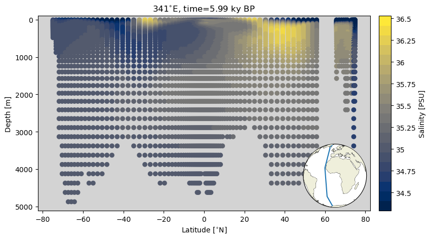
Section: lat or lon v. depth#
A section plot is a depth transect in which the x axis reflects a distance metric (latitude or longitude in this case), the y axis is depth with some variable plotted as color. Here we will plot the data as a scatterplot, and then as filled contour plot. The calculations involved in producing filled contour plots require the data be more regular. because we are selecting data along a line of longitude, we can describe our coordinates with a vector of latitude values and a vector of depth values–the true tenants of a grid!
As a nice bit of convenience, we introduce an inset map that makes it easier to contextualize the depth transect.
lims = [340, 342]
_sect_ds = dp.between(subarea_ds, 'TLONG', lims)
sect_ds = _sect_ds[var].squeeze()
sect_ds = sect_ds.compute()

lat_lims = [min(sect_ds.TLAT.mean(dim='nlon')), max(sect_ds.TLAT.mean(dim='nlon'))]
lon_lims = np.mean(lims)*np.ones(2)
def make_inset_map(ax, lats, lons, central_lon=0,central_lat=0, size_scaler=.25, loc="lower right"):
    axin = inset_axes(ax, width=size_scaler*5, height=size_scaler*5, loc=loc,
                 axes_class=cartopy.mpl.geoaxes.GeoAxes,
                 axes_kwargs=dict(projection=ccrs.Orthographic(central_latitude=central_lat,
                                                               central_longitude=central_lon)))
                                                               # central_lon)))

    axin.coastlines(linewidth=.5)
    axin.add_feature(cfeature.LAND, zorder=14)
    axin.plot(lons, lats, transform=ccrs.PlateCarree())
    axin.set_global()
From now on, make_inset_map will be loaded from plotting_helpers.
fig = plt.figure(figsize=(9,5));
gs = gridspec.GridSpec(1, 2, wspace=0.05, width_ratios=[8, .3])
ax = fig.add_subplot(gs[0, 0]);
ax.patch.set_facecolor('lightgray')

ax.contourf(sect_ds.TLAT.mean(dim='nlon'), sect_ds.z_t_m,
                     sect_ds.mean(dim='nlon').squeeze().data,10, origin='upper',
                         levels=ax2_levels,
                         cmap=ax2_sm.cmap,
                        norm=ax2_sm.norm)


ylims = ax.get_ylim()
ax.set_ylim([ylims[1], ylims[0]])
ax.set_ylabel('Depth [m]')
ax.set_xlabel('Latitude [{}]'.format(lat_u))

ax2_cb = fig.add_subplot(gs[0, 1])
cb2 = plt.colorbar(ax2_sm,cax=ax2_cb, orientation='vertical',label='Salinity [{}]'.format(colorbar_units),
                   format=FormatStrFormatter('%g'))

make_inset_map(ax, lat_lims, lon_lims, central_lon=0,central_lat=0)
ax.set_title('{}{}, time={} {}'.format(341,lon_u, time, time_u));
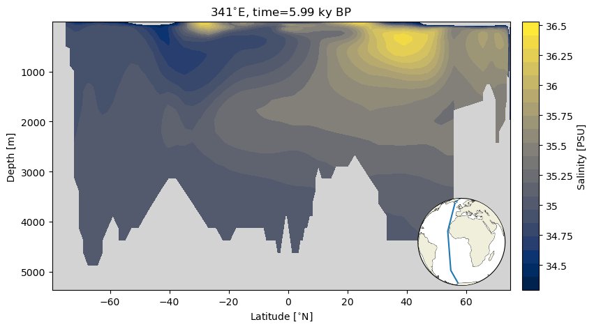
fig = plt.figure(figsize=(9,5));
gs = gridspec.GridSpec(1, 2, wspace=0.05, width_ratios=[8, .3])
ax = fig.add_subplot(gs[0, 0]);
# background color
ax.patch.set_facecolor('lightgray')

# for scatter, because color var is an array, need to make a mesh version of x and y vars
lat_mesh, depth_mesh = np.meshgrid(sect_ds.TLAT.mean(dim='nlon'), sect_ds.z_t_m)
ax.scatter(lat_mesh,depth_mesh,
                     c=sect_ds.mean(dim='nlon').squeeze().data,
                         cmap=ax2_sm.cmap,
                        norm=ax2_sm.norm)


ylims = ax.get_ylim()
ax.set_ylim([ylims[1], max([-100,ylims[0]])])
ax.set_ylabel('Depth [m]')
ax.set_xlabel('Latitude [{}]'.format(lat_u))

ax2_cb = fig.add_subplot(gs[0, 1])
cb2 = plt.colorbar(ax2_sm,cax=ax2_cb, orientation='vertical',label='Salinity [{}]'.format(colorbar_units),
                   format=FormatStrFormatter('%g'))

make_inset_map(ax, lat_lims, lon_lims, central_lon=0,central_lat=0)
ax.set_title('{}{}, time={} {}'.format(341,lon_u, time, time_u));
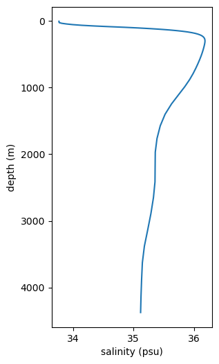
Profile: var 1 v. depth#
Last plot type! We are frequently interested in how some variable changes with depth. This is a little simpler on a regular grid when it is possible to query by dimensions. Instead, we’ll get as close as we can and then take the mean latitude-wise and then longitude-wise so we are left with a depth profile.
lims = [340, 342]
_sect_ds = dp.between(subarea_ds, 'TLONG', lims)
lims = [40, 42]
prof_reg = dp.between(_sect_ds['SALT'].squeeze(), 'TLAT', lims)
prof_reg = prof_reg.compute()
lat = prof_reg.TLAT.mean(dim='nlon')
lon = prof_reg.TLONG.mean(dim='nlat')
prof = prof_reg.mean(dim='nlat').mean(dim='nlon')
prof_df = pd.DataFrame({'values': prof.data, 'label': ['prof_1' for ik in range(len(prof.data))], 'depth': prof.z_t_m.data})
fig = plt.figure(figsize=(3,6));
ax = fig.add_subplot();

ax.plot('values', 'depth', data=prof_df)
ax.invert_yaxis()
ax.set_ylabel('depth (m)')
ax.set_xlabel('salinity (psu)')
Text(0.5, 0, 'salinity (psu)')
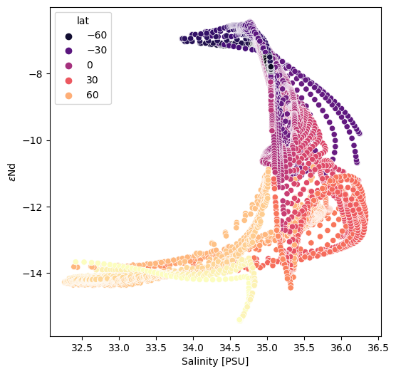
Scatter: var1 v. var2 (colored by var3)#
While we have discussed scatter plots before, let’s have a quick look at the case in which the x and y values are variable rather than positional.
Seaborn is such user friendly tool for this sort of thing that it is silly not to leverage it. That said, it doesn’t take in xarray datasets (yet!), so we’ll need to do a little data restructuring.
It appears (as far as this author can tell), that filtering an xarray dataset applies a mask to the array, but does not filter the scope of the coordinates. For illustrative purposes, we want to have latitude, longitude and depth available as variables so we need to cajol them into the same shape as, for example, SALT.
make longitude, latitude and depth arrays that each have the same three dimensional size (corresponding to the dimensions of the target variable, e.g., SALT)
longmesh = np.array([_sect_ds.TLONG.data for ik in range(len(_sect_ds.z_t_m))])
latmesh = np.array([_sect_ds.TLAT.data for ik in range(len(_sect_ds.z_t_m))])
depthmesh = np.array([depth*np.ones_like(_sect_ds.TLONG.data) for depth in _sect_ds.z_t_m.data])
build a boolean filter to identify the nan values in the SALT array (these correspond to landmasses and the data that were masked earlier because they didn’t fall on the line of longitude we specified)
nan_filter = np.isnan(_sect_ds['SALT'].data)
filter all arrays with the
.isnan()filter
filtered_salt = _sect_ds['SALT'].data[~nan_filter].compute()
filtered_eNd = _sect_ds['eNd'].data[~nan_filter].compute()

filtered_lon = longmesh[~nan_filter]
filtered_lat = latmesh[~nan_filter]
filtered_depth = depthmesh[~nan_filter]
/Users/jlanders/opt/miniconda3/envs/paleobook-dev/lib/python3.10/site-packages/dask/core.py:119: RuntimeWarning: invalid value encountered in divide
  return func(*(_execute_task(a, cache) for a in args))
package all these neatly constructed arrays into a dataframe!
sect_df = pd.DataFrame({'salt':filtered_salt.ravel(),'eNd':filtered_eNd.ravel(),
                   'lon':filtered_lon.ravel(),
                   'lat':filtered_lat.ravel(), 'depth':filtered_depth.ravel()})
fig = plt.figure(figsize=(6,6))
ax = fig.add_subplot()
sns.scatterplot(x='salt', y='eNd', hue='lat', data=sect_df, palette='magma')
ax.set_ylabel(eNd_label)
ax.set_xlabel('Salinity [PSU]')
Text(0.5, 0, 'Salinity [PSU]')
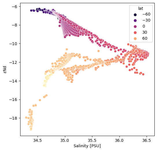
surf_df = pd.DataFrame({'lon': surf_ds.TLONG.data.ravel(), 'lat': surf_ds.TLAT.data.ravel(), 'eNd': surf_ds['eNd'].data.ravel(), 'salt': surf_ds['SALT'].data.ravel()})
surf_df = surf_df.dropna()
/Users/jlanders/opt/miniconda3/envs/paleobook-dev/lib/python3.10/site-packages/dask/core.py:119: RuntimeWarning: invalid value encountered in divide
  return func(*(_execute_task(a, cache) for a in args))
fig = plt.figure(figsize=(6,6))
ax = fig.add_subplot()
sns.scatterplot(x='salt', y='eNd', hue='lat', data=surf_df, palette='magma', ax=ax)
ax.set_ylabel(eNd_label)
ax.set_xlabel('Salinity [PSU]');
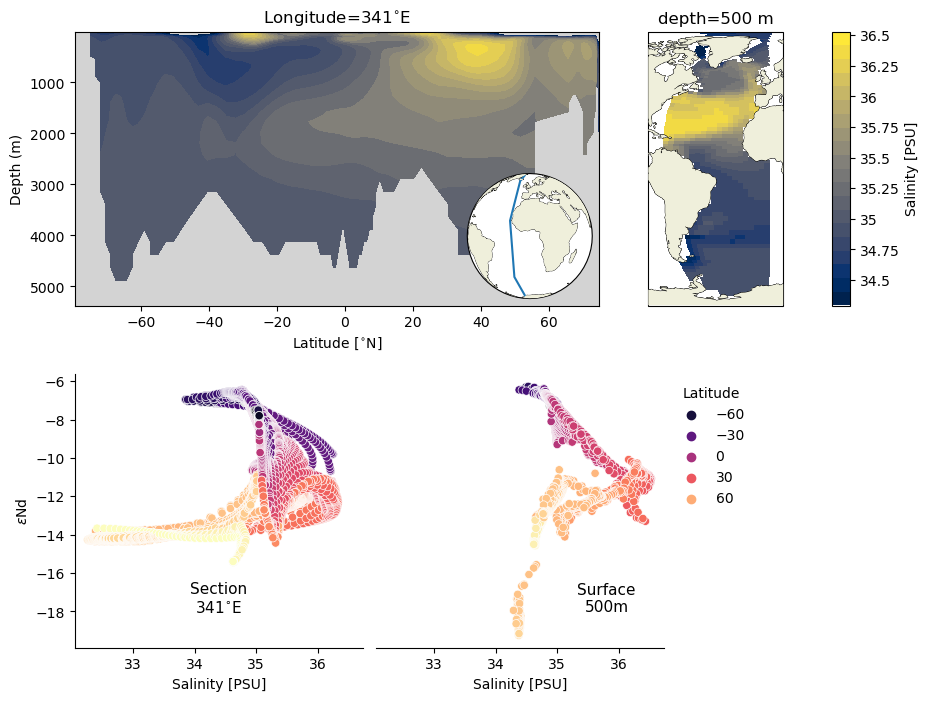
Dashboard#
Finally, we can pull all of these elements together in a dashboard.
fig = plt.figure(figsize=(10,8));
gs0 = fig.add_gridspec(2, 1, hspace=.25)

gs1 = gs0[0].subgridspec(1, 3, wspace=0, width_ratios=[9, 4,.3])
sect_ax = fig.add_subplot(gs1[0])
surf_ax = fig.add_subplot(gs1[1], projection=ccrs.Robinson(central_longitude=0))
cb_sal = fig.add_subplot(gs1[2])

# section plot
sect_ax.patch.set_facecolor('lightgray')
sect_ax.contourf(sect_ds.TLAT.mean(dim='nlon'), sect_ds.z_t_m,
                     sect_ds.mean(dim='nlon').squeeze().data,10, origin='upper',
                         levels=ax2_levels,
                         cmap=ax2_sm.cmap,
                        norm=ax2_sm.norm)


ylims = sect_ax.get_ylim()
sect_ax.set_ylim([ylims[1], max([-100,ylims[0]])])
sect_ax.set_ylabel('Depth (m)')
sect_ax.set_xlabel('Latitude [{}]'.format(lat_u))
sect_ax.set_title('Longitude=341{}'.format(lon_u))

make_inset_map(sect_ax, lat_lims, lon_lims, central_lon=0,central_lat=0)

# surface plot
c_snapshot_data_surf.plot.pcolormesh(ax=surf_ax,
                                   transform=ccrs.PlateCarree(),
                                   x='TLONG', y='TLAT',
                                   levels=ax2_levels,
                                  cmap=cf2_kwargs['cmap'],
                                  norm=cf2_kwargs['norm'],
                                  add_colorbar=False);

surf_ax.add_feature(cfeature.COASTLINE, edgecolor='k',linewidth=.5)
surf_ax.set_extent([lonlims[0]-10,lonlims[1]+10, latlims[0], latlims[1]], crs=ccrs.PlateCarree())
surf_ax.coastlines(linewidth=.5)
surf_ax.add_feature(cfeature.LAND, zorder=14)
surf_ax.set_title('depth=500 m')

# colorbar
cb2 = plt.colorbar(ax2_sm,cax=cb_sal, orientation='vertical',label='Salinity [{}]'.format(colorbar_units),
                   format=FormatStrFormatter('%g'))

# scatter plots
gs2 = gs0[1].subgridspec(1, 3, wspace=0.05, width_ratios=[5, 5, 3])
sect_scatter_ax = fig.add_subplot(gs2[0])
surf_scatter_ax = fig.add_subplot(gs2[1], sharex=sect_scatter_ax)
sns.scatterplot(x='salt', y='eNd', hue='lat', data=surf_df, ax=surf_scatter_ax, palette='magma')
sns.scatterplot(x='salt', y='eNd', hue='lat', data=sect_df, ax=sect_scatter_ax, palette='magma',legend=False)
surf_scatter_ax.legend(title='Latitude',frameon=False,bbox_to_anchor=(1,1), loc="upper left")

ylims = surf_scatter_ax.get_ylim()
sect_scatter_ax.set_ylim(ylims)

surf_scatter_ax.spines['right'].set_visible(False)
sect_scatter_ax.spines['right'].set_visible(False)
surf_scatter_ax.spines['top'].set_visible(False)
sect_scatter_ax.spines['top'].set_visible(False)
surf_scatter_ax.spines['left'].set_visible(False)

surf_scatter_ax.set_yticks([])
surf_scatter_ax.set_ylabel('')
sect_scatter_ax.set_ylabel(eNd_label)
surf_scatter_ax.set_xlabel('Salinity [PSU]')
sect_scatter_ax.set_xlabel('Salinity [PSU]')

left, width = .25, .5
bottom, height = .25, .5
right = left + width
top = bottom + height

sect_scatter_ax.text(0.5*(left+right), 0.18*(bottom+top), 'Section\n341{}'.format(lon_u),
        horizontalalignment='center',
        verticalalignment='center',
        fontsize=11, color='black',
        transform=sect_scatter_ax.transAxes)

surf_scatter_ax.text(0.8*(left+right), 0.18*(bottom+top), 'Surface\n500m',
        horizontalalignment='center',
        verticalalignment='center',
        fontsize=11, color='black',
        transform=surf_scatter_ax.transAxes)
Text(0.8, 0.18, 'Surface\n500m')
Summary#
There are a myriad of ways to combine these plots to build a story, but these examples should serve as solid starting points for each figure type.
Resources and references#
Citations |
|---|
Gu, Sifan, Liu, Zhengyu, Jahn, Alexandra, Zanowski, Hannah. (2021). C-iTRACE. Version 1.0. UCAR/NCAR - DASH Repository. https://doi.org/10.5065/hanq-bn92. |
Schlitzer, Reiner, Ocean Data View, odv.awi.de, 2023. |