Assembling the proxy database from the LiPDVerse

Assembling the proxy database from the LiPDVerse#

⚠️ Warning

This notebook contains a cell that starts a widget to help with identifying duplicates in the database. We strongly advise that you do not run the widget yourself unless you intend to go through the cleaning process. A list of removed datasets (TSiDS) and the reason they were removed or kept is stored in csv files in this repository. The resulting cleaned database has also been saved in a pickle file.

❗ DO NOT RUN ALL!!!!!!

Authors#

Deborah Khider & Julien Emile-Geay

Goal#

The goal of this notebook is to showcase data querying on the LiPDverser to create the proxy database

Data Description#

This notebook makes use of the LiPDVerse database, which contains datasets from various working groups. For a list of these compilations, see this page.

In particular, we will be using PAGES2kTemperature, iso-2k, and CoralHydro2k compilations for this demonstration.

PAGES2k: PAGES2k Consortium., Emile-Geay, J., McKay, N. et al. A global multiproxy database for temperature reconstructions of the Common Era. Sci Data 4, 170088 (2017). doi:10.1038/sdata.2017.88
iso2k: Konecky, B. L., McKay, N. P., Churakova (Sidorova), O. V., Comas-Bru, L., Dassié, E. P., DeLong, K. L., Falster, G. M., Fischer, M. J., Jones, M. D., Jonkers, L., Kaufman, D. S., Leduc, G., Managave, S. R., Martrat, B., Opel, T., Orsi, A. J., Partin, J. W., Sayani, H. R., Thomas, E. K., Thompson, D. M., Tyler, J. J., Abram, N. J., Atwood, A. R., Cartapanis, O., Conroy, J. L., Curran, M. A., Dee, S. G., Deininger, M., Divine, D. V., Kern, Z., Porter, T. J., Stevenson, S. L., von Gunten, L., and Iso2k Project Members: The Iso2k database: a global compilation of paleo-δ18O and δ2H records to aid understanding of Common Era climate, Earth Syst. Sci. Data, 12, 2261–2288, https://doi.org/10.5194/essd-12-2261-2020, 2020.
CoralHydro2k: Walter, R. M., H. R. Sayani, T. Felis, K. M. Cobb, N. J. Abram, A. K. Arzey, A. R. Atwood, L. D. Brenner, E. P. Dassi ́e, K. L. DeLong, B. Ellis, J. Emile-Geay, M. J. Fischer, N. F. Goodkin, J. A. Hargreaves, K. H. Kilbourne, H. Krawczyk, N. P. McKay, A. L. Moore, S. A. Murty, M. R. Ong, R. D. Ramos, E. V. Reed, D. Samanta, S. C. Sanchez, J. Zinke, and the PAGES CoralHydro2k Project Members (2023), The CoralHydro2k database: a global, actively curated compilation of coral δ18O and Sr / Ca proxy records of tropical ocean hydrology and temperature for the Common Era, Earth System Science Data, 15(5), 2081–2116, doi:10.5194/essd-15-2081-2023.

Let’s start by downloading the datasets.

⚠️ Warning: You only need to run the cell below once. It will download the data locally. The rest of the notebook assumes that the data is organized according to the output of the cell below.

# URL Links to download the data

pages2k_url = "https://lipdverse.org/Pages2kTemperature/current_version/Pages2kTemperature2_2_0.zip"
iso2k_url = "https://lipdverse.org/iso2k/current_version/iso2k1_1_2.zip"
coral2k_url ="https://lipdverse.org/CoralHydro2k/current_version/CoralHydro2k1_0_1.zip"

urls = [pages2k_url,iso2k_url,coral2k_url]
folders = ['Pages2k', 'iso2k', 'coral2k']

# import the necessary packages
import os
import requests
import zipfile
from pathlib import Path

## PAGES2k
# Define folder path and URL
for idx,url in enumerate(urls):
    folder_path = Path(f"./data/{folders[idx]}")
    zip_path = folder_path.with_suffix('.zip')

    # Step 1: Check if folder exists, create if not
    folder_path.mkdir(parents=True, exist_ok=True)

    # Step 2: Check if folder is empty
    if not any(folder_path.iterdir()):
        print("Folder is empty. Downloading data...")

        # Step 3: Download zip file
        response = requests.get(url)
        with open(zip_path, 'wb') as f:
            f.write(response.content)
        print(f"Downloaded ZIP to {zip_path}")

        # Step 4: Extract zip contents into folder
        with zipfile.ZipFile(zip_path, 'r') as zip_ref:
            zip_ref.extractall(folder_path)
        print(f"Extracted contents to {folder_path}")

Folder is empty. Downloading data...
Downloaded ZIP to data/Pages2k.zip
Extracted contents to data/Pages2k
Folder is empty. Downloading data...
Downloaded ZIP to data/iso2k.zip
Extracted contents to data/iso2k
Folder is empty. Downloading data...
Downloaded ZIP to data/coral2k.zip
Extracted contents to data/coral2k

Exploring the records in each of the compilations#

Let’s start with importing the needed packages:

import os

# General data manipulation libraries
import numpy as np
import pandas as pd

# To manipulate LiPD files
from pylipd.lipd import LiPD
import json

# Scientific toolboxes
import pyleoclim as pyleo
import seaborn as sns
import cfr
from scipy import stats

#To be able to compare timeseries
from scipy.stats import zscore
from dtaidistance import dtw
from scipy.stats import pearsonr, zscore
import matplotlib.pyplot as plt
import itertools

#For saving
import pickle

PAGES2k#

Let’s start with the PAGES2k dataset. We can load the entire folder into a pylipd.LiPD object:

D_pages2k = LiPD()
D_pages2k.load_from_dir('./data/Pages2k/')

Loading 647 LiPD files

100%|██████████| 647/647 [00:11<00:00, 54.47it/s]

Loaded..

Let’s create a query to gather all the necessary information. Since PyLiPD is build upon the rdflib library and LiPD is defined as a child of the Graph class in rdflib, it is possible to directly query a LiPD object using a SPARQL query as in this tutorial:

query = """ PREFIX le: <http://linked.earth/ontology#>
PREFIX wgs84: <http://www.w3.org/2003/01/geo/wgs84_pos#>
PREFIX rdfs: <http://www.w3.org/2000/01/rdf-schema#>

SELECT ?dataSetName ?compilationName ?archiveType ?geo_meanLat ?geo_meanLon ?geo_meanElev 
    ?paleoData_variableName ?paleoData_standardName ?paleoData_values ?paleoData_units 
    ?paleoData_proxy ?paleoData_proxyGeneral ?paleoData_seasonality ?paleoData_interpName ?paleoData_interpRank 
    ?TSID ?time_variableName ?time_standardName ?time_values
	?time_units where{
    
    ?ds a le:Dataset .
    ?ds le:hasName ?dataSetName .

    # Get the archive
    OPTIONAL{
            ?ds le:hasArchiveType ?archiveTypeObj .
            ?archiveTypeObj rdfs:label ?archiveType .
        }
    
    # Geographical information    
    
    ?ds le:hasLocation ?loc .
        OPTIONAL{?loc wgs84:lat ?geo_meanLat .}
        OPTIONAL{?loc wgs84:long ?geo_meanLon .}      
        OPTIONAL{?loc wgs84:alt ?geo_meanElev .}
    
    # PaleoData

    ?ds le:hasPaleoData ?data .
    ?data le:hasMeasurementTable ?table .
    ?table le:hasVariable ?var .

    # Name
    ?var le:hasName ?paleoData_variableName .
    ?var le:hasStandardVariable ?variable_obj .
    ?variable_obj rdfs:label ?paleoData_standardName .
    
    #Values
    ?var le:hasValues ?paleoData_values .

    #Seasonality
    OPTIONAL{?var le:seasonality ?paleoData_seasonality} .

    #Units
    OPTIONAL{
        ?var le:hasUnits ?paleoData_unitsObj .
        ?paleoData_unitsObj rdfs:label ?paleoData_units .
    }

    #Proxy information
    OPTIONAL{
        ?var le:hasProxy ?paleoData_proxyObj .
        ?paleoData_proxyObj rdfs:label ?paleoData_proxy .
    }
    OPTIONAL{
        ?var le:hasProxyGeneral ?paleoData_proxyGeneralObj .
        ?paleoData_proxyGeneralObj rdfs:label ?paleoData_proxyGeneral .
    }

    # Compilation
    ?var le:partOfCompilation ?compilation . 
    ?compilation le:hasName ?compilationName .
    FILTER (?compilationName = "Pages2kTemperature").
    ?var le:useInGlobalTemperatureAnalysis True .

    # TSiD (should all have them)
    OPTIONAL{
        ?var le:hasVariableId ?TSID
    } .

    # Interpretation (might be an optional field)
    OPTIONAL{
        ?var le:hasInterpretation ?interp .

        ?interp le:hasVariable ?interpvar .
        BIND(REPLACE(STR(?interpvar), "http://linked.earth/ontology/interpretation#", "") AS ?interpretedVariable_Fallback)
        OPTIONAL { ?interpvar rdfs:label ?interpretedVariable_Label } # Use a temporary variable for the label
        BIND(COALESCE(?interpretedVariable_Label, ?interpretedVariable_Fallback) AS ?paleoData_interpName) # COALESCE into the final variable
        }
    
    OPTIONAL{
        ?var le:hasInterpretation ?interp .
        ?interp le:hasRank ?paleoData_interpRank .}
    
    
    OPTIONAL{
        ?var le:hasInterpretation ?interp .
    
        ?interp le:hasSeasonality ?seasonalityURI .
        BIND(REPLACE(STR(?seasonalityURI), "http://linked.earth/ontology/interpretation#", "") AS ?seasonality_Fallback)
        OPTIONAL { ?seasonalityURI rdfs:label ?seasonalityLabel }
        BIND(COALESCE(?seasonalityLabel, ?seasonality_Fallback) AS ?paleoData_seasonality)
    }

    #Time information
    ?table le:hasVariable ?timevar .
    ?timevar le:hasName ?time_variableName .
    ?timevar le:hasStandardVariable ?timevar_obj .
    ?timevar_obj rdfs:label ?time_standardName .
    VALUES ?time_standardName {"year"} .
    ?timevar le:hasValues ?time_values .
    OPTIONAL{
        ?timevar le:hasUnits ?time_unitsObj .
        ?time_unitsObj rdfs:label ?time_units .
    }  
}"""

qres, df_pages2k = D_pages2k.query(query)
df_pages2k.head()

	dataSetName	compilationName	archiveType	geo_meanLat	geo_meanLon	geo_meanElev	paleoData_variableName	paleoData_standardName	paleoData_values	paleoData_units	paleoData_proxy	paleoData_proxyGeneral	paleoData_seasonality	paleoData_interpName	paleoData_interpRank	TSID	time_variableName	time_standardName	time_values	time_units
0	Ant-WDC05A.Steig.2013	Pages2kTemperature	Glacier ice	-79.46	-112.09	1806.0	d18O	d18O	[-33.32873325, -35.6732, -33.1574, -34.2854, -...	permil	d18O	None	Annual	temperature	NaN	Ant_030	year	year	[2005, 2004, 2003, 2002, 2001, 2000, 1999, 199...	yr AD
1	NAm-MtLemon.Briffa.2002	Pages2kTemperature	Wood	32.50	-110.80	2700.0	MXD	MXD	[0.968, 0.962, 1.013, 0.95, 1.008, 0.952, 1.02...	None	maximum latewood density	dendrophysical	Summer	temperature	NaN	NAm_568	year	year	[1568, 1569, 1570, 1571, 1572, 1573, 1574, 157...	yr AD
2	Arc-Arjeplog.Bjorklund.2014	Pages2kTemperature	Wood	66.30	18.20	800.0	density	density	[-0.829089212152348, -0.733882889924006, -0.89...	None	maximum latewood density	dendrophysical	Jun-Aug	temperature	NaN	Arc_060	year	year	[1200, 1201, 1202, 1203, 1204, 1205, 1206, 120...	yr AD
3	Asi-CHIN019.Li.2010	Pages2kTemperature	Wood	29.15	99.93	2150.0	ringWidth	ringWidth	[1.465, 1.327, 1.202, 0.757, 1.094, 1.006, 1.2...	None	ring width	dendrophysical	Annual	temperature	NaN	Asia_041	year	year	[1509, 1510, 1511, 1512, 1513, 1514, 1515, 151...	yr AD
4	NAm-Landslide.Luckman.2006	Pages2kTemperature	Wood	60.20	-138.50	800.0	ringWidth	ringWidth	[1.123, 0.841, 0.863, 1.209, 1.139, 1.056, 0.8...	None	ring width	dendrophysical	Summer	temperature	NaN	NAm_1876	year	year	[913, 914, 915, 916, 917, 918, 919, 920, 921, ...	yr AD

Let’s have a look at the resulting data.

df_pages2k.info()

<class 'pandas.core.frame.DataFrame'>
RangeIndex: 691 entries, 0 to 690
Data columns (total 20 columns):
 #   Column                  Non-Null Count  Dtype  
---  ------                  --------------  -----  
 dataSetName             691 non-null    object 
 compilationName         691 non-null    object 
 archiveType             691 non-null    object 
 geo_meanLat             691 non-null    float64
 geo_meanLon             691 non-null    float64
 geo_meanElev            684 non-null    float64
 paleoData_variableName  691 non-null    object 
 paleoData_standardName  691 non-null    object 
 paleoData_values        691 non-null    object 
 paleoData_units         283 non-null    object 
paleoData_proxy         691 non-null    object 
paleoData_proxyGeneral  500 non-null    object 
paleoData_seasonality   691 non-null    object 
paleoData_interpName    691 non-null    object 
paleoData_interpRank    1 non-null      float64
TSID                    691 non-null    object 
time_variableName       691 non-null    object 
time_standardName       691 non-null    object 
time_values             691 non-null    object 
time_units              691 non-null    object 
dtypes: float64(4), object(16)
memory usage: 108.1+ KB

df_pages2k['paleoData_interpName'].unique()

array(['temperature'], dtype=object)

We have 691 timeseries that represent temperature, consistent with the information from the LiPDverse.

iso2k#

Let’s do something similar for the iso2k database:

D_iso2k = LiPD()
D_iso2k.load_from_dir('./data/iso2k')

Loading 509 LiPD files

100%|██████████| 509/509 [00:14<00:00, 34.94it/s]

Loaded..

query_iso = """ PREFIX le: <http://linked.earth/ontology#>
PREFIX wgs84: <http://www.w3.org/2003/01/geo/wgs84_pos#>
PREFIX rdfs: <http://www.w3.org/2000/01/rdf-schema#>

SELECT ?dataSetName ?compilationName ?archiveType ?geo_meanLat ?geo_meanLon ?geo_meanElev 
    ?paleoData_variableName ?paleoData_standardName ?paleoData_values ?paleoData_units 
    ?paleoData_proxy ?paleoData_proxyGeneral ?paleoData_seasonality ?paleoData_interpName ?paleoData_interpRank 
    ?TSID ?time_variableName ?time_standardName ?time_values
	?time_units where{
    
    ?ds a le:Dataset .
    ?ds le:hasName ?dataSetName .

    # Get the archive
    OPTIONAL{
            ?ds le:hasArchiveType ?archiveTypeObj .
            ?archiveTypeObj rdfs:label ?archiveType .
        }
    
    # Geographical information    
    
    ?ds le:hasLocation ?loc .
        OPTIONAL{?loc wgs84:lat ?geo_meanLat .}
        OPTIONAL{?loc wgs84:long ?geo_meanLon .}      
        OPTIONAL{?loc wgs84:alt ?geo_meanElev .}
    
    # PaleoData

    ?ds le:hasPaleoData ?data .
    ?data le:hasMeasurementTable ?table .
    ?table le:hasVariable ?var .

    # Name
    ?var le:hasName ?paleoData_variableName .
    ?var le:hasStandardVariable ?variable_obj .
    ?variable_obj rdfs:label ?paleoData_standardName .
    
    #Values
    ?var le:hasValues ?paleoData_values .

    #Seasonality
    OPTIONAL{?var le:seasonality ?paleoData_seasonality} .

    #Units
    OPTIONAL{
        ?var le:hasUnits ?paleoData_unitsObj .
        ?paleoData_unitsObj rdfs:label ?paleoData_units .
    }

    #Proxy information
    OPTIONAL{
        ?var le:hasProxy ?paleoData_proxyObj .
        ?paleoData_proxyObj rdfs:label ?paleoData_proxy .
    }
    OPTIONAL{
        ?var le:hasProxyGeneral ?paleoData_proxyGeneralObj .
        ?paleoData_proxyGeneralObj rdfs:label ?paleoData_proxyGeneral .
    }

    # Compilation
    ?var le:partOfCompilation ?compilation . 
    ?compilation le:hasName ?compilationName .
    FILTER (?compilationName = "iso2k").
    ?var le:useInGlobalTemperatureAnalysis True .

    # TSiD (should all have them)
    OPTIONAL{
        ?var le:hasVariableId ?TSID
    } .

    # Interpretation (might be an optional field)
    OPTIONAL{
        ?var le:hasInterpretation ?interp .

        ?interp le:hasVariable ?interpvar .
        BIND(REPLACE(STR(?interpvar), "http://linked.earth/ontology/interpretation#", "") AS ?interpretedVariable_Fallback)
        OPTIONAL { ?interpvar rdfs:label ?interpretedVariable_Label } # Use a temporary variable for the label
        BIND(COALESCE(?interpretedVariable_Label, ?interpretedVariable_Fallback) AS ?paleoData_interpName) # COALESCE into the final variable
        }
    
    OPTIONAL{
        ?var le:hasInterpretation ?interp .
        ?interp le:hasRank ?paleoData_interpRank .}
    
    
    OPTIONAL{
        ?var le:hasInterpretation ?interp .
    
        ?interp le:hasSeasonality ?seasonalityURI .
        BIND(REPLACE(STR(?seasonalityURI), "http://linked.earth/ontology/interpretation#", "") AS ?seasonality_Fallback)
        OPTIONAL { ?seasonalityURI rdfs:label ?seasonalityLabel }
        BIND(COALESCE(?seasonalityLabel, ?seasonality_Fallback) AS ?paleoData_seasonality)
    }

    #Time information
    ?table le:hasVariable ?timevar .
    ?timevar le:hasName ?time_variableName .
    ?timevar le:hasStandardVariable ?timevar_obj .
    ?timevar_obj rdfs:label ?time_standardName .
    VALUES ?time_standardName {"year"} .
    ?timevar le:hasValues ?time_values .
    OPTIONAL{
        ?timevar le:hasUnits ?time_unitsObj .
        ?time_unitsObj rdfs:label ?time_units .
    }  
}"""

qres, df_iso2k = D_iso2k.query(query_iso)
df_iso2k.head()

	dataSetName	compilationName	archiveType	geo_meanLat	geo_meanLon	geo_meanElev	paleoData_variableName	paleoData_standardName	paleoData_values	paleoData_units	paleoData_proxy	paleoData_proxyGeneral	paleoData_seasonality	paleoData_interpName	paleoData_interpRank	TSID	time_variableName	time_standardName	time_values	time_units
0	LS16STCL	iso2k	Lake sediment	50.830	-116.39	1126.0	d18O	d18O	[-7.81, -5.91, -9.03, -5.35, -5.61, -5.98, -5....	permil	d18O	None	Winter	effectivePrecipitation	NaN	LPD7dc5b9ba-dup-dup	year	year	[2009.0, 2008.3, 2007.8, 2007.4, 2007.0, 2006....	yr AD
1	LS16STCL	iso2k	Lake sediment	50.830	-116.39	1126.0	d18O	d18O	[-7.81, -5.91, -9.03, -5.35, -5.61, -5.98, -5....	permil	d18O	None	None	effectivePrecipitation	3.0	LPD7dc5b9ba-dup-dup	year	year	[2009.0, 2008.3, 2007.8, 2007.4, 2007.0, 2006....	yr AD
2	CO00URMA	iso2k	Coral	0.933	173.00	6.0	d18O	d18O	[-4.8011, -4.725, -4.6994, -4.86, -5.0886, -5....	permil	d18O	None	subannual	temperature	1.0	Ocean2kHR_177_iso2k	year	year	[1994.5, 1994.33, 1994.17, 1994.0, 1993.83, 19...	yr AD
3	CO00URMA	iso2k	Coral	0.933	173.00	6.0	d18O	d18O	[-4.8011, -4.725, -4.6994, -4.86, -5.0886, -5....	permil	d18O	None	subannual	temperature	1.0	Ocean2kHR_177_iso2k	year	year	[1994.5, 1994.33, 1994.17, 1994.0, 1993.83, 19...	yr AD
4	CO00URMA	iso2k	Coral	0.933	173.00	6.0	d18O	d18O	[-4.8011, -4.725, -4.6994, -4.86, -5.0886, -5....	permil	d18O	None	subannual	temperature	1.0	Ocean2kHR_177_iso2k	year	year	[1994.5, 1994.33, 1994.17, 1994.0, 1993.83, 19...	yr AD

df_iso2k['paleoData_interpName'].unique()

array(['effectivePrecipitation', 'temperature', 'seawaterIsotope',
       'precipitationIsotope', 'hydrologicBalance', 'salinity'],
      dtype=object)

Despite using the useinGlobalTemperatureAnalysis flag, there seems to be more than 1 interpretation for several of the variables. Let’s first filer for interpretation associated with temperature and remove duplicate entries based on TSiD:

df_iso2k_filt = df_iso2k[df_iso2k['paleoData_interpName']=='temperature'].drop_duplicates(subset='TSID', keep='first')
df_iso2k_filt.head()

	dataSetName	compilationName	archiveType	geo_meanLat	geo_meanLon	geo_meanElev	paleoData_variableName	paleoData_standardName	paleoData_values	paleoData_units	paleoData_proxy	paleoData_proxyGeneral	paleoData_seasonality	paleoData_interpName	paleoData_interpRank	TSID	time_variableName	time_standardName	time_values	time_units
2	CO00URMA	iso2k	Coral	0.9330	173.0000	6.0	d18O	d18O	[-4.8011, -4.725, -4.6994, -4.86, -5.0886, -5....	permil	d18O	None	subannual	temperature	1.0	Ocean2kHR_177_iso2k	year	year	[1994.5, 1994.33, 1994.17, 1994.0, 1993.83, 19...	yr AD
11	CO05KUBE	iso2k	Coral	32.4670	-64.7000	-12.0	d18O	d18O	[-4.15, -3.66, -3.69, -4.07, -3.95, -4.12, -3....	permil	d18O	None	subannual	temperature	1.0	Ocean2kHR_105_iso2k	year	year	[1983.21, 1983.13, 1983.04, 1982.96, 1982.88, ...	yr AD
13	IC13THQU	iso2k	Glacier ice	-13.9333	-70.8333	5670.0	d18O	d18O	[-18.5905, -16.3244, -16.2324, -17.0112, -18.6...	permil	d18O	None	Winter	temperature	NaN	SAm_035_iso2k	year	year	[2009, 2008, 2007, 2006, 2005, 2004, 2003, 200...	yr AD
15	CO01TUNG	iso2k	Coral	-5.2170	145.8170	-3.0	d18O	d18O	[-4.875, -4.981, -5.166, -5.06, -4.942, -4.919...	permil	d18O	None	subannual	temperature	NaN	Ocean2kHR_141_iso2k	year	year	[1993.042, 1992.792, 1992.542, 1992.292, 1992....	yr AD
19	CO01TUNG	iso2k	Coral	-5.2170	145.8170	-3.0	d18O	d18O	[-4.827, -4.786, -4.693, -4.852, -4.991, -4.90...	permil	d18O	None	subannual	temperature	1.0	Ocean2kHR_140_iso2k	year	year	[1993.042, 1992.792, 1992.542, 1992.292, 1992....	yr AD

df_iso2k_filt.info()

<class 'pandas.core.frame.DataFrame'>
Index: 49 entries, 2 to 155
Data columns (total 20 columns):
 #   Column                  Non-Null Count  Dtype  
---  ------                  --------------  -----  
 dataSetName             49 non-null     object 
 compilationName         49 non-null     object 
 archiveType             49 non-null     object 
 geo_meanLat             49 non-null     float64
 geo_meanLon             49 non-null     float64
 geo_meanElev            49 non-null     float64
 paleoData_variableName  49 non-null     object 
 paleoData_standardName  49 non-null     object 
 paleoData_values        49 non-null     object 
 paleoData_units         49 non-null     object 
paleoData_proxy         49 non-null     object 
paleoData_proxyGeneral  0 non-null      object 
paleoData_seasonality   39 non-null     object 
paleoData_interpName    49 non-null     object 
paleoData_interpRank    24 non-null     float64
TSID                    49 non-null     object 
time_variableName       49 non-null     object 
time_standardName       49 non-null     object 
time_values             49 non-null     object 
time_units              49 non-null     object 
dtypes: float64(4), object(16)
memory usage: 8.0+ KB

We have 49 entries left in the iso2k database.

CoralHydro2k#

Let’s repeat our filtering. The CoralHydro2k database does not have a property indicating whether to use in temperature analysis.

D_coral2k = LiPD()
D_coral2k.load_from_dir('./data/coral2k')

Loading 179 LiPD files

100%|██████████| 179/179 [00:02<00:00, 88.65it/s]

Loaded..

query_coral = """ PREFIX le: <http://linked.earth/ontology#>
PREFIX wgs84: <http://www.w3.org/2003/01/geo/wgs84_pos#>
PREFIX rdfs: <http://www.w3.org/2000/01/rdf-schema#>

SELECT ?dataSetName ?compilationName ?archiveType ?geo_meanLat ?geo_meanLon ?geo_meanElev 
    ?paleoData_variableName ?paleoData_standardName ?paleoData_values ?paleoData_units 
    ?paleoData_proxy ?paleoData_proxyGeneral ?paleoData_seasonality ?paleoData_interpName ?paleoData_interpRank 
    ?TSID ?time_variableName ?time_standardName ?time_values
	?time_units where{
    
    ?ds a le:Dataset .
    ?ds le:hasName ?dataSetName .

    # Get the archive
    OPTIONAL{
            ?ds le:hasArchiveType ?archiveTypeObj .
            ?archiveTypeObj rdfs:label ?archiveType .
        }
    
    # Geographical information    
    
    ?ds le:hasLocation ?loc .
        OPTIONAL{?loc wgs84:lat ?geo_meanLat .}
        OPTIONAL{?loc wgs84:long ?geo_meanLon .}      
        OPTIONAL{?loc wgs84:alt ?geo_meanElev .}
    
    # PaleoData

    ?ds le:hasPaleoData ?data .
    ?data le:hasMeasurementTable ?table .
    ?table le:hasVariable ?var .

    # Name
    ?var le:hasName ?paleoData_variableName .
    ?var le:hasStandardVariable ?variable_obj .
    ?variable_obj rdfs:label ?paleoData_standardName .
    
    #Values
    ?var le:hasValues ?paleoData_values .

    #Seasonality
    OPTIONAL{?var le:seasonality ?paleoData_seasonality} .

    #Units
    OPTIONAL{
        ?var le:hasUnits ?paleoData_unitsObj .
        ?paleoData_unitsObj rdfs:label ?paleoData_units .
    }

    #Proxy information
    OPTIONAL{
        ?var le:hasProxy ?paleoData_proxyObj .
        ?paleoData_proxyObj rdfs:label ?paleoData_proxy .
    }
    OPTIONAL{
        ?var le:hasProxyGeneral ?paleoData_proxyGeneralObj .
        ?paleoData_proxyGeneralObj rdfs:label ?paleoData_proxyGeneral .
    }

    # Compilation
    ?var le:partOfCompilation ?compilation . 
    ?compilation le:hasName ?compilationName .
    FILTER (?compilationName = "CoralHydro2k").


    # TSiD (should all have them)
    OPTIONAL{
        ?var le:hasVariableId ?TSID
    } .

    # Interpretation (might be an optional field)
    OPTIONAL{
        ?var le:hasInterpretation ?interp .

        ?interp le:hasVariable ?interpvar .
        BIND(REPLACE(STR(?interpvar), "http://linked.earth/ontology/interpretation#", "") AS ?interpretedVariable_Fallback)
        OPTIONAL { ?interpvar rdfs:label ?interpretedVariable_Label } # Use a temporary variable for the label
        BIND(COALESCE(?interpretedVariable_Label, ?interpretedVariable_Fallback) AS ?paleoData_interpName) # COALESCE into the final variable
        }
    
    OPTIONAL{
        ?var le:hasInterpretation ?interp .
        ?interp le:hasRank ?paleoData_interpRank .}
    
    
    OPTIONAL{
        ?var le:hasInterpretation ?interp .
    
        ?interp le:hasSeasonality ?seasonalityURI .
        BIND(REPLACE(STR(?seasonalityURI), "http://linked.earth/ontology/interpretation#", "") AS ?seasonality_Fallback)
        OPTIONAL { ?seasonalityURI rdfs:label ?seasonalityLabel }
        BIND(COALESCE(?seasonalityLabel, ?seasonality_Fallback) AS ?paleoData_seasonality)
    }

    #Time information
    ?table le:hasVariable ?timevar .
    ?timevar le:hasName ?time_variableName .
    ?timevar le:hasStandardVariable ?timevar_obj .
    ?timevar_obj rdfs:label ?time_standardName .
    VALUES ?time_standardName {"year"} .
    ?timevar le:hasValues ?time_values .
    OPTIONAL{
        ?timevar le:hasUnits ?time_unitsObj .
        ?time_unitsObj rdfs:label ?time_units .
    }  
}"""

qres, df_coral2k = D_coral2k.query(query_coral)
df_coral2k.head()

	dataSetName	compilationName	archiveType	geo_meanLat	geo_meanLon	geo_meanElev	paleoData_variableName	paleoData_standardName	paleoData_values	paleoData_units	paleoData_proxy	paleoData_proxyGeneral	paleoData_seasonality	paleoData_interpName	paleoData_interpRank	TSID	time_variableName	time_standardName	time_values	time_units
0	KA17RYU01	CoralHydro2k	Coral	28.300	130.000	-3.5	SrCa	Sr/Ca	[8.802, 9.472, 8.825, 9.355, 8.952, 9.297, 8.8...	mmol/mol	None	None	None	None	None	KA17RYU01_SrCa	year	year	[1578.58, 1579.08, 1579.58, 1580.08, 1580.58, ...	yr AD
1	CH18YOA02	CoralHydro2k	Coral	16.448	111.605	NA	SrCa	Sr/Ca	[8.58, 8.683, 8.609, 8.37, 8.38, 8.417, 8.584,...	mmol/mol	None	None	None	None	None	CH18YOA02_SrCa	year	year	[1987.92, 1988.085, 1988.25, 1988.42, 1988.585...	yr AD
2	FL17DTO02	CoralHydro2k	Coral	24.699	-82.799	-3.0	SrCa	Sr/Ca	[9.159, 9.257, 9.245, 9.166, 9.045, 9.013, 8.9...	mmol/mol	None	None	None	None	None	FL17DTO02_SrCa	year	year	[1837.04, 1837.13, 1837.21, 1837.29, 1837.38, ...	yr AD
3	BO14HTI01	CoralHydro2k	Coral	12.210	109.310	-3.6	d18O	d18O	[-5.4206, -5.3477, -5.1354, -5.7119, -5.9058, ...	permil	None	None	None	None	None	BO14HTI01_d18O	year	year	[1977.37, 1977.45, 1977.54, 1977.62, 1977.7, 1...	yr AD
4	BO14HTI01	CoralHydro2k	Coral	12.210	109.310	-3.6	SrCa	Sr/Ca	[9.2, 9.17, 9.11, 9.02, 8.95, 8.99, 9.06, 9.1,...	mmol/mol	None	None	None	None	None	BO14HTI01_SrCa	year	year	[1600.04, 1600.12, 1600.2, 1600.28, 1600.37, 1...	yr AD

Since there is no interpretation objects to go by, let’s have a look at the names of the variables:

df_coral2k['paleoData_variableName'].unique()

array(['SrCa', 'd18O', 'd18O_sw'], dtype=object)

Sr/Ca is usually interpreted as a temperature proxy. d18O contains information about both temperature and d18Osw. Let’s keep these two and drop any duplicates as identified by TSiDs:

df_coral2k_filt = df_coral2k[df_coral2k['paleoData_variableName'].isin(['SrCa', 'd18O'])].drop_duplicates(subset='TSID', keep='first')
df_coral2k_filt.head()

	dataSetName	compilationName	archiveType	geo_meanLat	geo_meanLon	geo_meanElev	paleoData_variableName	paleoData_standardName	paleoData_values	paleoData_units	paleoData_proxy	paleoData_proxyGeneral	paleoData_seasonality	paleoData_interpName	paleoData_interpRank	TSID	time_variableName	time_standardName	time_values	time_units
0	KA17RYU01	CoralHydro2k	Coral	28.300	130.000	-3.5	SrCa	Sr/Ca	[8.802, 9.472, 8.825, 9.355, 8.952, 9.297, 8.8...	mmol/mol	None	None	None	None	None	KA17RYU01_SrCa	year	year	[1578.58, 1579.08, 1579.58, 1580.08, 1580.58, ...	yr AD
1	CH18YOA02	CoralHydro2k	Coral	16.448	111.605	NA	SrCa	Sr/Ca	[8.58, 8.683, 8.609, 8.37, 8.38, 8.417, 8.584,...	mmol/mol	None	None	None	None	None	CH18YOA02_SrCa	year	year	[1987.92, 1988.085, 1988.25, 1988.42, 1988.585...	yr AD
2	FL17DTO02	CoralHydro2k	Coral	24.699	-82.799	-3.0	SrCa	Sr/Ca	[9.159, 9.257, 9.245, 9.166, 9.045, 9.013, 8.9...	mmol/mol	None	None	None	None	None	FL17DTO02_SrCa	year	year	[1837.04, 1837.13, 1837.21, 1837.29, 1837.38, ...	yr AD
3	BO14HTI01	CoralHydro2k	Coral	12.210	109.310	-3.6	d18O	d18O	[-5.4206, -5.3477, -5.1354, -5.7119, -5.9058, ...	permil	None	None	None	None	None	BO14HTI01_d18O	year	year	[1977.37, 1977.45, 1977.54, 1977.62, 1977.7, 1...	yr AD
4	BO14HTI01	CoralHydro2k	Coral	12.210	109.310	-3.6	SrCa	Sr/Ca	[9.2, 9.17, 9.11, 9.02, 8.95, 8.99, 9.06, 9.1,...	mmol/mol	None	None	None	None	None	BO14HTI01_SrCa	year	year	[1600.04, 1600.12, 1600.2, 1600.28, 1600.37, 1...	yr AD

df_coral2k_filt.info()

<class 'pandas.core.frame.DataFrame'>
Index: 233 entries, 0 to 251
Data columns (total 20 columns):
 #   Column                  Non-Null Count  Dtype  
---  ------                  --------------  -----  
 dataSetName             233 non-null    object 
 compilationName         233 non-null    object 
 archiveType             233 non-null    object 
 geo_meanLat             233 non-null    float64
 geo_meanLon             233 non-null    float64
 geo_meanElev            232 non-null    object 
 paleoData_variableName  233 non-null    object 
 paleoData_standardName  233 non-null    object 
 paleoData_values        233 non-null    object 
 paleoData_units         233 non-null    object 
paleoData_proxy         0 non-null      object 
paleoData_proxyGeneral  0 non-null      object 
paleoData_seasonality   0 non-null      object 
paleoData_interpName    0 non-null      object 
paleoData_interpRank    0 non-null      object 
TSID                    233 non-null    object 
time_variableName       233 non-null    object 
time_standardName       233 non-null    object 
time_values             233 non-null    object 
time_units              233 non-null    object 
dtypes: float64(2), object(18)
memory usage: 38.2+ KB

This database adds 233 new records.

DataBase: Assemble!#

Let’s concatenate the three DataFrames into a clean database, dropping timeseries with the same TSiD as we go. Let’s also convert the values to numpy.array:

df_raw = pd.concat([df_pages2k, df_iso2k_filt, df_coral2k_filt], ignore_index=True).drop_duplicates(subset='TSID', keep='first')
df_raw['paleoData_values']=df_raw['paleoData_values'].apply(lambda row : json.loads(row) if isinstance(row, str) else row)
df_raw['time_values']=df_raw['time_values'].apply(lambda row : json.loads(row) if isinstance(row, str) else row)
df_raw.info()

<class 'pandas.core.frame.DataFrame'>
Index: 972 entries, 0 to 972
Data columns (total 20 columns):
 #   Column                  Non-Null Count  Dtype  
---  ------                  --------------  -----  
 dataSetName             972 non-null    object 
 compilationName         972 non-null    object 
 archiveType             972 non-null    object 
 geo_meanLat             972 non-null    float64
 geo_meanLon             972 non-null    float64
 geo_meanElev            964 non-null    object 
 paleoData_variableName  972 non-null    object 
 paleoData_standardName  972 non-null    object 
 paleoData_values        972 non-null    object 
 paleoData_units         564 non-null    object 
paleoData_proxy         739 non-null    object 
paleoData_proxyGeneral  500 non-null    object 
paleoData_seasonality   729 non-null    object 
paleoData_interpName    739 non-null    object 
paleoData_interpRank    24 non-null     float64
TSID                    972 non-null    object 
time_variableName       972 non-null    object 
time_standardName       972 non-null    object 
time_values             972 non-null    object 
time_units              972 non-null    object 
dtypes: float64(3), object(17)
memory usage: 159.5+ KB

We have 972 timeseries before any further pre-processing.

Special handling: The Palmyra record#

The Palmyra Coral record in these databases may not have been updated with the latest changes published by Dee et al. (2020). Let’s open this record and extract the same information:

palm = LiPD()
palm.load('./data/Palmyra.Dee.2020.lpd')

Loading 1 LiPD files

100%|██████████| 1/1 [00:00<00:00,  9.18it/s]

Loaded..

query_palm = """
PREFIX le: <http://linked.earth/ontology#>
PREFIX wgs84: <http://www.w3.org/2003/01/geo/wgs84_pos#>
PREFIX rdfs: <http://www.w3.org/2000/01/rdf-schema#>

SELECT ?dataSetName ?compilationName ?archiveType ?geo_meanLat ?geo_meanLon ?geo_meanElev 
    ?paleoData_variableName ?paleoData_standardName ?paleoData_values ?paleoData_units 
    ?paleoData_proxy ?paleoData_proxyGeneral ?paleoData_seasonality ?paleoData_interpName ?paleoData_interpRank 
    ?TSID ?time_variableName ?time_standardName ?time_values
	?time_units where{
    
    ?ds a le:Dataset .
    ?ds le:hasName ?dataSetName .

    # Get the archive
    OPTIONAL{
            ?ds le:hasArchiveType ?archiveTypeObj .
            ?archiveTypeObj rdfs:label ?archiveType .
        }
    
    # Geographical information    
    
    ?ds le:hasLocation ?loc .
        OPTIONAL{?loc wgs84:lat ?geo_meanLat .}
        OPTIONAL{?loc wgs84:long ?geo_meanLon .}      
        OPTIONAL{?loc wgs84:alt ?geo_meanElev .}
    
    # PaleoData

    ?ds le:hasPaleoData ?data .
    ?data le:hasMeasurementTable ?table .
    ?table le:hasVariable ?var .

    # Name
    ?var le:hasName ?paleoData_variableName .
    ?var le:hasStandardVariable ?variable_obj .
    ?variable_obj rdfs:label ?paleoData_standardName .
    
    #Values
    ?var le:hasValues ?paleoData_values .

    #Units
    OPTIONAL{
        ?var le:hasUnits ?paleoData_unitsObj .
        ?paleoData_unitsObj rdfs:label ?paleoData_units .
    }

    #Proxy information
    OPTIONAL{
        ?var le:hasProxy ?paleoData_proxyObj .
        ?paleoData_proxyObj rdfs:label ?paleoData_proxy .
    }
    OPTIONAL{
        ?var le:hasProxyGeneral ?paleoData_proxyGeneralObj .
        ?paleoData_proxyGeneralObj rdfs:label ?paleoData_proxyGeneral .
    }

    # Compilation
    OPTIONAL{
    ?var le:partOfCompilation ?compilation . 
    ?compilation le:hasName ?compilationName .}


    # TSiD (should all have them)
    OPTIONAL{
        ?var le:hasVariableId ?TSID
    } .

    # Interpretation (might be an optional field)
    OPTIONAL{
        ?var le:hasInterpretation ?interp .

        ?interp le:hasVariable ?interpvar .
        BIND(REPLACE(STR(?interpvar), "http://linked.earth/ontology/interpretation#", "") AS ?interpretedVariable_Fallback)
        OPTIONAL { ?interpvar rdfs:label ?interpretedVariable_Label } # Use a temporary variable for the label
        BIND(COALESCE(?interpretedVariable_Label, ?interpretedVariable_Fallback) AS ?paleoData_interpName) # COALESCE into the final variable
        }
    
    OPTIONAL{
        ?var le:hasInterpretation ?interp .
        ?interp le:hasRank ?paleoData_interpRank .}
    
    
    OPTIONAL{
        ?var le:hasInterpretation ?interp .
    
        ?interp le:hasSeasonality ?seasonalityURI .
        BIND(REPLACE(STR(?seasonalityURI), "http://linked.earth/ontology/interpretation#", "") AS ?seasonality_Fallback)
        OPTIONAL { ?seasonalityURI rdfs:label ?seasonalityLabel }
        BIND(COALESCE(?seasonalityLabel, ?seasonality_Fallback) AS ?paleoData_seasonality)
    }

    #Time information
    ?table le:hasVariable ?timevar .
    ?timevar le:hasName ?time_variableName .
    ?timevar le:hasStandardVariable ?timevar_obj .
    ?timevar_obj rdfs:label ?time_standardName .
    VALUES ?time_standardName {"year"} .
    ?timevar le:hasValues ?time_values .
    OPTIONAL{
        ?timevar le:hasUnits ?time_unitsObj .
        ?time_unitsObj rdfs:label ?time_units .
    }  
}"""

qres, df_palm = palm.query(query_palm)
df_palm.head()

	dataSetName	compilationName	archiveType	geo_meanLat	geo_meanLon	geo_meanElev	paleoData_variableName	paleoData_standardName	paleoData_values	paleoData_units	paleoData_proxy	paleoData_proxyGeneral	paleoData_seasonality	paleoData_interpName	paleoData_interpRank	TSID	time_variableName	time_standardName	time_values	time_units
0	Palmyra.Dee.2020	None	Coral	5.8664	-162.12	-9.0	d18O	d18O	[-4.749, -4.672, -4.724, -4.717, -4.8947, -4.8...	permil	d18O	isotopic	subannual	seawaterIsotope	1.0	PCU-1cce3af5639a4ec	year	year	[1146.375, 1146.4583, 1146.5417, 1146.625, 114...	yr AD
1	Palmyra.Dee.2020	None	Coral	5.8664	-162.12	-9.0	d18O	d18O	[-4.749, -4.672, -4.724, -4.717, -4.8947, -4.8...	permil	d18O	isotopic	subannual	temperature	NaN	PCU-1cce3af5639a4ec	year	year	[1146.375, 1146.4583, 1146.5417, 1146.625, 114...	yr AD
2	Palmyra.Dee.2020	None	Coral	5.8664	-162.12	-9.0	year	year	[1146.375, 1146.4583, 1146.5417, 1146.625, 114...	yr AD	None	None	None	None	NaN	PCU-45b2ff49e3944f1	year	year	[1146.375, 1146.4583, 1146.5417, 1146.625, 114...	yr AD

Let’s keep the variable associated with the temperature interpretation:

df_palm_filt = df_palm[df_palm['paleoData_interpName']=='temperature']
df_palm_filt

	dataSetName	compilationName	archiveType	geo_meanLat	geo_meanLon	geo_meanElev	paleoData_variableName	paleoData_standardName	paleoData_values	paleoData_units	paleoData_proxy	paleoData_proxyGeneral	paleoData_seasonality	paleoData_interpName	paleoData_interpRank	TSID	time_variableName	time_standardName	time_values	time_units
1	Palmyra.Dee.2020	None	Coral	5.8664	-162.12	-9.0	d18O	d18O	[-4.749, -4.672, -4.724, -4.717, -4.8947, -4.8...	permil	d18O	isotopic	subannual	temperature	NaN	PCU-1cce3af5639a4ec	year	year	[1146.375, 1146.4583, 1146.5417, 1146.625, 114...	yr AD

Let’s make sure that all the values are converted from string:

df_palm_filt['paleoData_values']=df_palm_filt['paleoData_values'].apply(lambda row : json.loads(row) if isinstance(row, str) else row)
df_palm_filt['time_values']=df_palm_filt['time_values'].apply(lambda row : json.loads(row) if isinstance(row, str) else row)

Handling duplication: Sr/Ca#

Now, let’s find the entry(ies) within PAGES2k corresponding to the Palmyra record. To do so, let’s find all the records within 50km:

# Earth's radius in kilometers
R = 6371.0

# Threshold
threshold = 50 #Look for all records within threshold km

# Target location
target_lat = df_palm_filt['geo_meanLat'].iloc[0]
target_lon = df_palm_filt['geo_meanLon'].iloc[0]

# Convert degrees to radians
lat1 = np.radians(target_lat)
lon1 = np.radians(target_lon)
lat2 = np.radians(df_raw['geo_meanLat'])
lon2 = np.radians(df_raw['geo_meanLon'])

# Haversine formula
dlat = lat2 - lat1
dlon = lon2 - lon1
a = np.sin(dlat / 2)**2 + np.cos(lat1) * np.cos(lat2) * np.sin(dlon / 2)**2
c = 2 * np.arcsin(np.sqrt(a))
distance_km = R * c

# Add distance column
df_raw['distance_km'] = distance_km

# Filter to only rows within 50 km
df_distance = df_raw[df_raw['distance_km'] <= threshold].reset_index(drop=True)
df_distance

	dataSetName	compilationName	archiveType	geo_meanLat	geo_meanLon	geo_meanElev	paleoData_variableName	paleoData_standardName	paleoData_values	paleoData_units	...	paleoData_proxyGeneral	paleoData_seasonality	paleoData_interpName	paleoData_interpRank	TSID	time_variableName	time_standardName	time_values	time_units	distance_km
0	Ocn-Palmyra.Nurhati.2011	Pages2kTemperature	Coral	5.870	-162.130	-10.0	Sr/Ca	Sr/Ca	[8.96, 8.9, 8.91, 8.94, 8.92, 8.89, 8.87, 8.81...	mmol/mol	...	None	subannual	temperature	NaN	Ocean2kHR_161	year	year	[1998.29, 1998.21, 1998.13, 1998.04, 1997.96, ...	yr AD	1.176328
1	Ocn-Palmyra.Cobb.2013	Pages2kTemperature	Coral	5.870	-162.130	-7.0	d18O	d18O	[-4.651, -4.631, -4.629, -4.562, -4.58, -4.442...	permil	...	None	subannual	temperature	NaN	Ocean2kHR_139	year	year	[928.125, 928.209, 928.292, 928.375, 928.459, ...	yr AD	1.176328
2	CO03COPM	iso2k	Coral	5.870	-162.130	-7.0	d18O	d18O	[-5.27, -5.42, -5.49, -5.5, -5.44, -5.48, -5.5...	permil	...	None	subannual	temperature	NaN	Ocean2kHR_139_iso2k	year	year	[1998.37, 1998.29, 1998.2, 1998.13, 1998.04, 1...	yr AD	1.176328
3	NU11PAL01	CoralHydro2k	Coral	5.867	-162.133	-9.0	d18O	d18O	[-4.79, -4.89, -4.81, -4.84, -4.85, -4.82, -4....	permil	...	None	None	None	NaN	NU11PAL01_d18O	year	year	[1886.13, 1886.21, 1886.29, 1886.38, 1886.46, ...	yr AD	1.439510
4	NU11PAL01	CoralHydro2k	Coral	5.867	-162.133	-9.0	SrCa	Sr/Ca	[9.01, 9.02, 8.98, 8.99, 9.0, 8.99, 9.0, 9.11,...	mmol/mol	...	None	None	None	NaN	NU11PAL01_SrCa	year	year	[1886.13, 1886.21, 1886.29, 1886.38, 1886.46, ...	yr AD	1.439510
5	SA19PAL01	CoralHydro2k	Coral	5.878	-162.142	-10.0	d18O	d18O	[-5.21, -5.23, -5.17, -5.13, -5.11, -5.05, -5....	permil	...	None	None	None	NaN	SA19PAL01_d18O	year	year	[1983.58, 1983.67, 1983.75, 1983.83, 1983.92, ...	yr AD	2.754166
6	SA19PAL01	CoralHydro2k	Coral	5.878	-162.142	-10.0	SrCa	Sr/Ca	[8.94, 9.08, 9.17, 9.16, 9.16, 9.17, 9.17, 9.1...	mmol/mol	...	None	None	None	NaN	SA19PAL01_SrCa	year	year	[1980.75, 1980.83, 1980.92, 1981.0, 1981.08, 1...	yr AD	2.754166
7	SA19PAL02	CoralHydro2k	Coral	5.878	-162.142	-10.0	d18O	d18O	[-5.05, -5.1, -5.21, -5.14, -5.23, -5.32, -5.3...	permil	...	None	None	None	NaN	SA19PAL02_d18O	year	year	[1985.92, 1986.0, 1986.08, 1986.17, 1986.25, 1...	yr AD	2.754166
8	SA19PAL02	CoralHydro2k	Coral	5.878	-162.142	-10.0	SrCa	Sr/Ca	[8.86, 8.82, 8.81, 8.85, 8.89, 8.87, 8.82, 8.8...	mmol/mol	...	None	None	None	NaN	SA19PAL02_SrCa	year	year	[1985.33, 1985.42, 1985.5, 1985.58, 1985.67, 1...	yr AD	2.754166
9	CO03PAL08	CoralHydro2k	Coral	5.870	-162.130	NA	d18O	d18O	[-5.14, -5.13, -5.13, -5.16, -5.28, -4.99, -4....	permil	...	None	None	None	NaN	CO03PAL08_d18O	year	year	[1653.63, 1653.65, 1653.686083, 1653.722167, 1...	yr AD	1.176328
10	CO03PAL09	CoralHydro2k	Coral	5.870	-162.130	NA	d18O	d18O	[-4.98, -4.8, -4.68, -4.74, -4.7, -4.74, -4.84...	permil	...	None	None	None	NaN	CO03PAL09_d18O	year	year	[1664.96, 1665.0215, 1665.083, 1665.164, 1665....	yr AD	1.176328
11	CO03PAL04	CoralHydro2k	Coral	5.870	-162.130	NA	d18O	d18O	[-4.86, -4.9, -5.0, -4.92, -4.91, -4.85, -4.74...	permil	...	None	None	None	NaN	CO03PAL04_d18O	year	year	[1398.68, 1398.747167, 1398.814333, 1398.8815,...	yr AD	1.176328
12	CO03PAL10	CoralHydro2k	Coral	5.870	-162.130	NA	d18O	d18O	[-4.865, -4.765, -4.805, -4.665, -4.595, -4.73...	permil	...	None	None	None	NaN	CO03PAL10_d18O	year	year	[1326.65, 1326.75825, 1326.8665, 1326.97475, 1...	yr AD	1.176328
13	CO03PAL05	CoralHydro2k	Coral	5.870	-162.130	NA	d18O	d18O	[-4.61, -4.64, -4.7, -4.77, -4.86, -4.85, -4.8...	permil	...	None	None	None	NaN	CO03PAL05_d18O	year	year	[1405.1569, 1405.280175, 1405.40345, 1405.5267...	yr AD	1.176328
14	CO03PAL07	CoralHydro2k	Coral	5.870	-162.130	NA	d18O	d18O	[-4.63, -4.55, -4.65, -4.59, -4.74, -4.79, -4....	permil	...	None	None	None	NaN	CO03PAL07_d18O	year	year	[1635.02, 1635.083, 1635.146, 1635.209, 1635.2...	yr AD	1.176328
15	CO03PAL06	CoralHydro2k	Coral	5.870	-162.130	NA	d18O	d18O	[-4.64, -4.64, -4.62, -4.62, -4.68, -4.77, -4....	permil	...	None	None	None	NaN	CO03PAL06_d18O	year	year	[1411.9262, 1412.0046, 1412.083, 1412.1775, 14...	yr AD	1.176328
16	CO03PAL02	CoralHydro2k	Coral	5.870	-162.130	NA	d18O	d18O	[-4.631, -4.724, -4.709, -4.707, -4.912, -4.83...	permil	...	None	None	None	NaN	CO03PAL02_d18O	year	year	[1149.08, 1149.2225, 1149.365, 1149.5075, 1149...	yr AD	1.176328
17	CO03PAL03	CoralHydro2k	Coral	5.870	-162.130	NA	d18O	d18O	[-4.79, -4.73, -4.66, -4.66, -4.78, -4.69, -4....	permil	...	None	None	None	NaN	CO03PAL03_d18O	year	year	[1317.17, 1317.29, 1317.41, 1317.53, 1317.65, ...	yr AD	1.176328
18	CO03PAL01	CoralHydro2k	Coral	5.870	-162.130	NA	d18O	d18O	[-4.68, -4.62, -4.65, -4.56, -4.58, -4.42, -4....	permil	...	None	None	None	NaN	CO03PAL01_d18O	year	year	[928.08, 928.175, 928.27, 928.365, 928.46, 928...	yr AD	1.176328

19 rows × 21 columns

The first 18 rows seem to be corresponding to various coral heads within the Palmyra records. Let’s have a look at them. Let’s first have a look at Sr/Ca record:

df_distance_SrCa = df_distance[df_distance['paleoData_variableName'].isin(['SrCa', 'Sr/Ca'])]
df_distance_SrCa

	dataSetName	compilationName	archiveType	geo_meanLat	geo_meanLon	geo_meanElev	paleoData_variableName	paleoData_standardName	paleoData_values	paleoData_units	...	paleoData_proxyGeneral	paleoData_seasonality	paleoData_interpName	paleoData_interpRank	TSID	time_variableName	time_standardName	time_values	time_units	distance_km
0	Ocn-Palmyra.Nurhati.2011	Pages2kTemperature	Coral	5.870	-162.130	-10.0	Sr/Ca	Sr/Ca	[8.96, 8.9, 8.91, 8.94, 8.92, 8.89, 8.87, 8.81...	mmol/mol	...	None	subannual	temperature	NaN	Ocean2kHR_161	year	year	[1998.29, 1998.21, 1998.13, 1998.04, 1997.96, ...	yr AD	1.176328
4	NU11PAL01	CoralHydro2k	Coral	5.867	-162.133	-9.0	SrCa	Sr/Ca	[9.01, 9.02, 8.98, 8.99, 9.0, 8.99, 9.0, 9.11,...	mmol/mol	...	None	None	None	NaN	NU11PAL01_SrCa	year	year	[1886.13, 1886.21, 1886.29, 1886.38, 1886.46, ...	yr AD	1.439510
6	SA19PAL01	CoralHydro2k	Coral	5.878	-162.142	-10.0	SrCa	Sr/Ca	[8.94, 9.08, 9.17, 9.16, 9.16, 9.17, 9.17, 9.1...	mmol/mol	...	None	None	None	NaN	SA19PAL01_SrCa	year	year	[1980.75, 1980.83, 1980.92, 1981.0, 1981.08, 1...	yr AD	2.754166
8	SA19PAL02	CoralHydro2k	Coral	5.878	-162.142	-10.0	SrCa	Sr/Ca	[8.86, 8.82, 8.81, 8.85, 8.89, 8.87, 8.82, 8.8...	mmol/mol	...	None	None	None	NaN	SA19PAL02_SrCa	year	year	[1985.33, 1985.42, 1985.5, 1985.58, 1985.67, 1...	yr AD	2.754166

4 rows × 21 columns

Let’s plot them:

ts_list = []
for _, row in df_distance_SrCa.iterrows():
    proxy = row['paleoData_proxy'] if isinstance(row['paleoData_proxy'],str) else row['paleoData_variableName']
    ts_list.append(pyleo.GeoSeries(time=row['time_values'],value=row['paleoData_values'],
                            time_name='Time',value_name=row['paleoData_variableName'],
                            time_unit=row['time_units'], value_unit=row['paleoData_units'],
                            lat = row['geo_meanLat'], lon = row['geo_meanLon'], 
                            elevation = row['geo_meanElev'], importedFrom='lipdverse.org',
                            archiveType = row['archiveType'],
                            observationType=row['paleoData_proxy'],       
                            label=row['dataSetName']+'_'+proxy, verbose = False)) 

mgs_srca = pyleo.MultipleGeoSeries(ts_list) 
fig, ax = mgs_srca.stackplot()
fig.show()

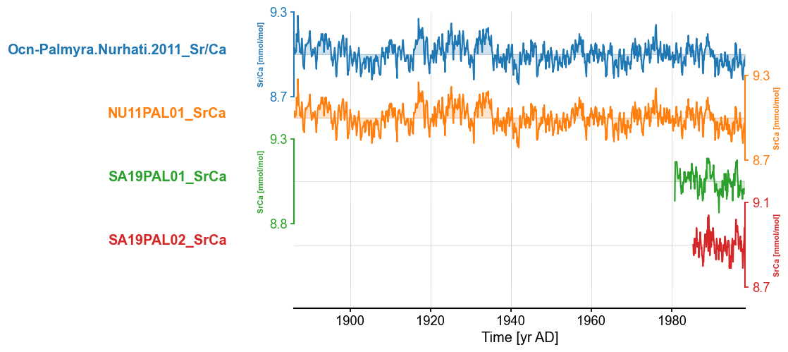
../../_images/c388ca6fc8d7e3de48d07e50ff1e017f7a7ef03b585e3137a3c695b217936e67.png

The three records look very similar. The Ocn-Palmyra.Nurhati.2011_Sr/Ca and NU11PAL01_SrCa appear nearly identical. However, this may occur in other places in the database, so we want an algorithm to (1) find records that may be the same. We can follow a similar strategy as we have done here. a. Are they within 50km of each other and b. do they have the same or similar variable names, and (2) assess whether these records are, in fact, the same.

We can do this in several ways:

Correlation: this may work well for true duplicates but may fail for composites
Dynamic Time Warping (DTW), which can be used to to assess shape similarity even when time points aren’t exactly aligned. DTW returns a distance metric: lower values mean more similar patterns.It can be combined with a z-normalization to remove mean/variance effects.
Principal Component Analysis (PCA)/ On groups of nearby records, run PCA to detect if certain records contribute nearly identical structure to the same components. High loadings on the same component can suggest redundancy.

Let’s have a look at these three options.

Option 1: Correlation#

Let’s use the Pyleoclim correlation function. The following code is inspired from this tutorial.

n = len(mgs_srca.series_list)
corr_mat = np.empty((n,n))
corr_mat[:] = np.nan #let's only work on half of the matrix to speeds things up

for i in range(0, n-1): # loop over records 
    ts = mgs_srca.series_list[i]    
    mgsl = pyleo.MultipleGeoSeries(mgs_srca.series_list[i+1:]) #gather potential pairs
    corr = mgsl.correlation(ts,method='built-in') # compute correlations
    corr_mat[i,i+1:] = corr.r # save result in matrix

Looping over 3 Series in collection

100%|██████████| 3/3 [00:00<00:00, 193.66it/s]

Looping over 2 Series in collection

100%|██████████| 2/2 [00:00<00:00, 288.76it/s]

Looping over 1 Series in collection

100%|██████████| 1/1 [00:00<00:00, 336.57it/s]

labels = []
for item in mgs_srca.series_list:
    labels.append(item.label)
core_matrix_df = pd.DataFrame(corr_mat, index=labels, columns=labels)
plt.figure(figsize=(10, 8))
sns.heatmap(core_matrix_df, annot=True, fmt=".2f", cmap="coolwarm", center=0)
plt.title("Correlation Heatmap")
plt.tight_layout()
plt.show()

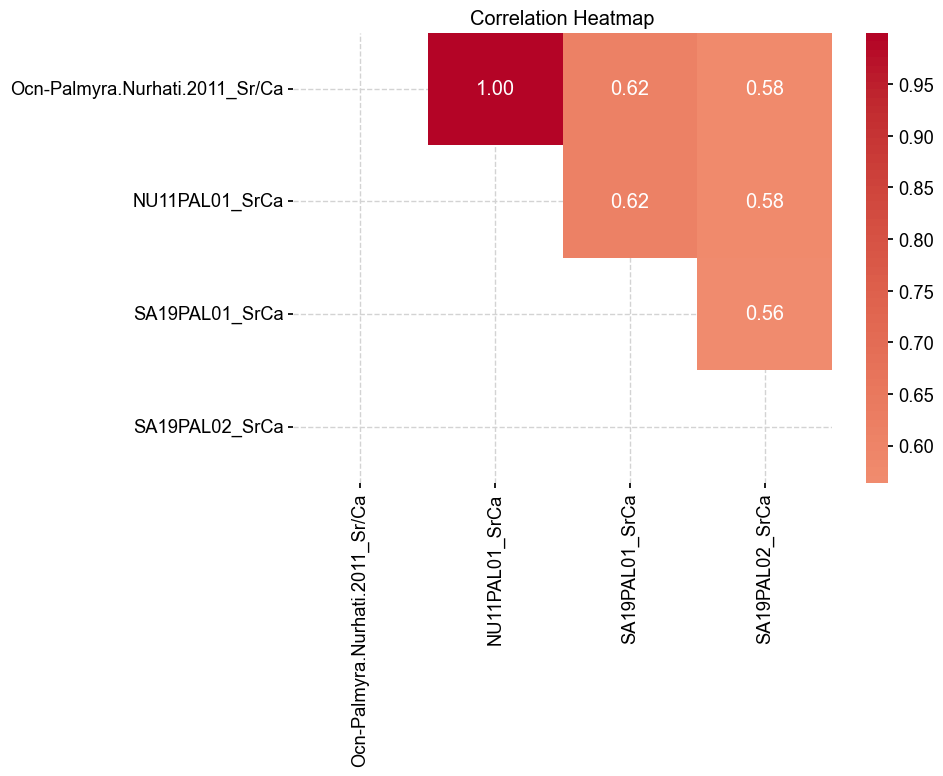
../../_images/73989ced1bc723539b77f1632034d0c38580dc036bb6d4761675b7ddc86375f3.png

Unsurprisingly, Ocn-Palmyra.Nurhati.2011_Sr/Ca and NU11PAL01_SrCa have a correlation of 1 as they are essentially the same record. The other correlations are below 0.8, which makes it difficult to assess whether they are, in fact the same record. Let’s have a look at DTW as a potential discriminant.

Option 2: Dynamic Time Wrapping#

Dynamic Time Wrapping (DTW) is a distance metric designed to compare time series that may be misaligned in time or differ in length. Unlike traditional correlation-based methods, DTW allows for flexible, non-linear alignment of sequences by warping the time axis to minimize the total distance between corresponding points. In our context, DTW provides a more robust measure of similarity between records than correlation, especially when records are composites or partially overlapping. By restricting comparisons to shared time intervals and z-score normalizing the data to emphasize shape similarity, DTW helps identify potentially redundant or duplicated records while accounting for the complexities inherent in paleoenvironmental data.

The following cell does the following:

Clip the timeseries for similar time range for comparison
Compute zscore
Compute the DTW distance

# --- Helper function: clip to overlapping time range and normalize ---

def clip_to_overlap(time1, series1, time2, series2, min_overlap=5):
    start = max(time1[0], time2[0])
    end = min(time1[-1], time2[-1])
    
    mask1 = (time1 >= start) & (time1 <= end)
    mask2 = (time2 >= start) & (time2 <= end)

    if np.sum(mask1) < min_overlap or np.sum(mask2) < min_overlap:
        return None, None  # Not enough overlapping points
    
    return zscore(series1[mask1]), zscore(series2[mask2])

# --- Prepare the data ----
records = {}
times = {}

for series in mgs_srca.series_list:
    records[series.label] = series.value
    times[series.label] = series.time


# --- Main loop ---
labels = list(records.keys())
n = len(labels)
dtw_matrix = np.full((n, n), np.nan)

for i, j in itertools.combinations(range(n), 2):
    key_i, key_j = labels[i], labels[j]

    s1, s2 = clip_to_overlap(times[key_i], records[key_i],
                             times[key_j], records[key_j])

    if s1 is not None:
        path = dtw.warping_path(s1, s2)
        dist = dtw.distance(s1, s2)
        norm_dist = dist / len(path)  # Per-step normalization

        dtw_matrix[i, j] = dtw_matrix[j, i] = norm_dist

# Convert to DataFrame for visualization
dtw_df = pd.DataFrame(dtw_matrix, index=labels, columns=labels)

Let’s visualize the results:

plt.figure(figsize=(10, 8))
sns.heatmap(dtw_df, annot=True, fmt=".2f", cmap="viridis", mask=np.isnan(dtw_df))
plt.title("DTW Distance Matrix (Clipped to Overlap)")
plt.tight_layout()
plt.show()

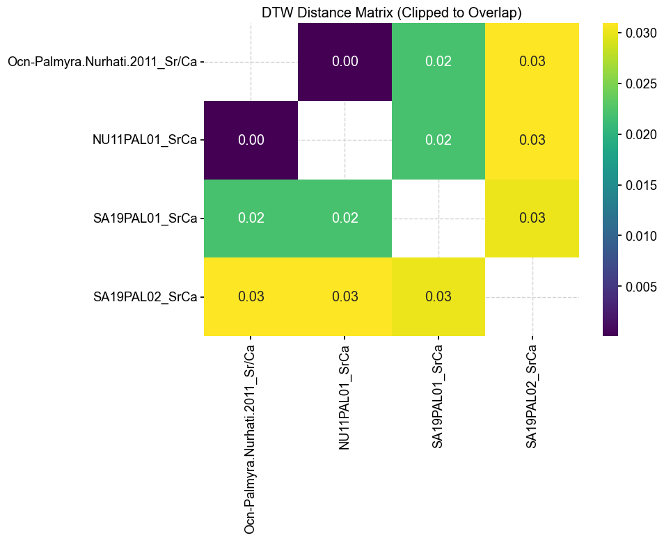
../../_images/f471fab3704dae64d775bd32ec3c269ae1ea433dbfd41ed2f79f8723d1030a92.png

The next problem lies in the interpretation of these results. The matrix holds pairwise DTW distances between time series. Each entry DTW[i, j] is a non-negative real number representing how similar two z-normalized time series are after optimal alignment.

Lower values = more similar shape (after warping).
Higher values = less similar (more misaligned or different structure).

Since we z-scored normalized the data and accounted for number of steps, the DTW distances can be interpreted as follows:

Normalized DTW	Meaning
0.0 – 0.1	Very similar shape — likely same core or duplicated segment
0.1 – 0.2	High similarity — possibly same site, maybe overlapping or composited
0.2 – 0.4	Moderate similarity — same region, but different signal characteristics
> 0.4	Different shape — likely independent records

Option 3: Principal Component Analysis#

Let’s leverage the PCA functionality in Pyleoclim. A tutorial for this functionality is available here.

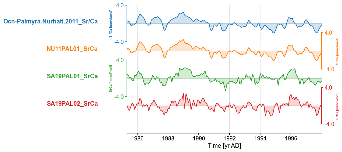
The first step is to brings the records on a common time axis and standardize them:

mgs_srca_sc = mgs_srca.common_time().standardize()
fig, ax = mgs_srca_sc.stackplot()

../../_images/37ac7c677e4abfef7af801b675839f1d8ba824d0b7f9c7eab8ab75c8ebe9ed5d.png

Let’s run PCA:

pca = mgs_srca_sc.pca()

And let’s have a look at the first mode:

fig, ax = pca.modeplot()

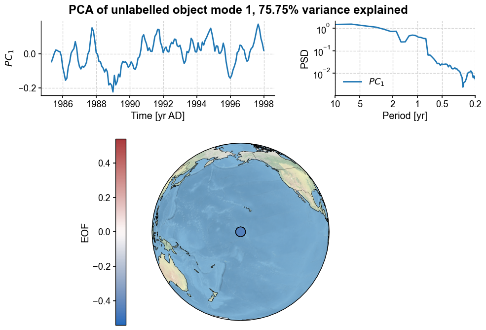
../../_images/711e097baa3f42b9f139df455a9aed2b15dbd981b1371133f66518ed6f9c1568.png

Not unsurprisingly, the first PC explains over 75% of the variance. Let’s have a look at the loads:

pca.eigvecs[1]

array([-0.54194915,  0.4525358 ,  0.03876175, -0.70710678])

The loads are not very similar, which is interesting considering that tow of these records are definitely the same. PCA may not work well to find duplicates.

Based on this small proof of concept, correlation and DTW seems to be a reasonable approach to identify duplicates in the database.

Handling duplication part 2: \(\delta^{18}\mathrm{O}\)#

Let’s now have a look at the various \(\delta^{18}\mathrm{O}\) records.

df_distance_d18O = df_distance[df_distance['paleoData_variableName']=='d18O']
df_distance_d18O.head()

	dataSetName	compilationName	archiveType	geo_meanLat	geo_meanLon	geo_meanElev	paleoData_variableName	paleoData_standardName	paleoData_values	paleoData_units	...	paleoData_proxyGeneral	paleoData_seasonality	paleoData_interpName	paleoData_interpRank	TSID	time_variableName	time_standardName	time_values	time_units	distance_km
1	Ocn-Palmyra.Cobb.2013	Pages2kTemperature	Coral	5.870	-162.130	-7.0	d18O	d18O	[-4.651, -4.631, -4.629, -4.562, -4.58, -4.442...	permil	...	None	subannual	temperature	NaN	Ocean2kHR_139	year	year	[928.125, 928.209, 928.292, 928.375, 928.459, ...	yr AD	1.176328
2	CO03COPM	iso2k	Coral	5.870	-162.130	-7.0	d18O	d18O	[-5.27, -5.42, -5.49, -5.5, -5.44, -5.48, -5.5...	permil	...	None	subannual	temperature	NaN	Ocean2kHR_139_iso2k	year	year	[1998.37, 1998.29, 1998.2, 1998.13, 1998.04, 1...	yr AD	1.176328
3	NU11PAL01	CoralHydro2k	Coral	5.867	-162.133	-9.0	d18O	d18O	[-4.79, -4.89, -4.81, -4.84, -4.85, -4.82, -4....	permil	...	None	None	None	NaN	NU11PAL01_d18O	year	year	[1886.13, 1886.21, 1886.29, 1886.38, 1886.46, ...	yr AD	1.439510
5	SA19PAL01	CoralHydro2k	Coral	5.878	-162.142	-10.0	d18O	d18O	[-5.21, -5.23, -5.17, -5.13, -5.11, -5.05, -5....	permil	...	None	None	None	NaN	SA19PAL01_d18O	year	year	[1983.58, 1983.67, 1983.75, 1983.83, 1983.92, ...	yr AD	2.754166
7	SA19PAL02	CoralHydro2k	Coral	5.878	-162.142	-10.0	d18O	d18O	[-5.05, -5.1, -5.21, -5.14, -5.23, -5.32, -5.3...	permil	...	None	None	None	NaN	SA19PAL02_d18O	year	year	[1985.92, 1986.0, 1986.08, 1986.17, 1986.25, 1...	yr AD	2.754166

5 rows × 21 columns

ts_list = []
for _, row in df_distance_d18O.iterrows():
    proxy = row['paleoData_proxy'] if isinstance(row['paleoData_proxy'],str) else row['paleoData_variableName']
    ts_list.append(pyleo.GeoSeries(time=row['time_values'],value=row['paleoData_values'],
                            time_name='Time',value_name=row['paleoData_variableName'],
                            time_unit=row['time_units'], value_unit=row['paleoData_units'],
                            lat = row['geo_meanLat'], lon = row['geo_meanLon'], 
                            elevation = row['geo_meanElev'], importedFrom='lipdverse.org',
                            archiveType = row['archiveType'],
                            observationType=row['paleoData_proxy'],       
                            label=row['dataSetName']+'_'+proxy, verbose = False)) 

# Add the Dee et al. record

ts_list.append(pyleo.GeoSeries(time=df_palm_filt['time_values'].iloc[0],
                    value=df_palm_filt['paleoData_values'].iloc[0],
                    time_name='Time',
                    value_name=df_palm_filt['paleoData_variableName'].iloc[0],
                    time_unit=df_palm_filt['time_units'].iloc[0], 
                    value_unit=df_palm_filt['paleoData_units'].iloc[0],
                    lat = df_palm_filt['geo_meanLat'].iloc[0],
                    lon = df_palm_filt['geo_meanLon'].iloc[0], 
                    elevation = df_palm_filt['geo_meanElev'].iloc[0],
                    importedFrom='lipdverse.org',
                    archiveType = df_palm_filt['archiveType'].iloc[0],
                    observationType=df_palm_filt['paleoData_proxy'].iloc[0],       
                    label=df_palm_filt['dataSetName'].iloc[0]+'_'+proxy, verbose = False))

mgs = pyleo.MultipleGeoSeries(ts_list) 
fig, ax = mgs.stackplot()

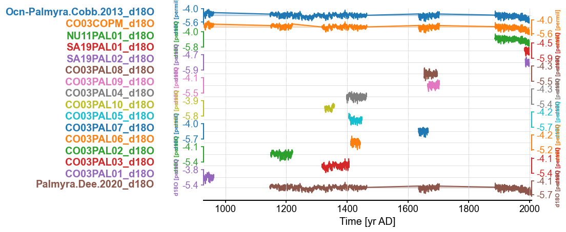
../../_images/16375f3fba15f44bd05bfe76123a205caf286a6b513b1f3c13cb1956e2835588.png

As we have seen with the Sr/Ca record, there seems to be duplications among the record. Although some look like changes in the age models. Let’s explore correlation and DTW to weed out the duplicates.

Option 1: Correlation#

n = len(mgs.series_list)
corr_mat = np.empty((n,n))
corr_mat[:] = np.nan #let's only work on half of the matrix to speeds things up

for i in range(0, n-1): # loop over records 
    ts = mgs.series_list[i]    
    mgsl = pyleo.MultipleGeoSeries(mgs.series_list[i+1:]) #gather potential pairs
    corr = mgsl.correlation(ts,method='built-in') # compute correlations
    corr_mat[i,i+1:] = corr.r # save result in matrix

Looping over 15 Series in collection

100%|██████████| 15/15 [00:00<00:00, 543.36it/s]

Looping over 14 Series in collection

100%|██████████| 14/14 [00:00<00:00, 612.66it/s]

Looping over 13 Series in collection

100%|██████████| 13/13 [00:00<00:00, 2594.87it/s]

Looping over 12 Series in collection

100%|██████████| 12/12 [00:00<00:00, 3536.76it/s]

Looping over 11 Series in collection

100%|██████████| 11/11 [00:00<00:00, 3804.83it/s]

Looping over 10 Series in collection

100%|██████████| 10/10 [00:00<00:00, 2108.33it/s]

Looping over 9 Series in collection

100%|██████████| 9/9 [00:00<00:00, 1791.42it/s]

Looping over 8 Series in collection

100%|██████████| 8/8 [00:00<00:00, 501.88it/s]

Looping over 7 Series in collection

100%|██████████| 7/7 [00:00<00:00, 980.70it/s]

Looping over 6 Series in collection

100%|██████████| 6/6 [00:00<00:00, 1411.43it/s]

Looping over 5 Series in collection

100%|██████████| 5/5 [00:00<00:00, 2103.25it/s]

Looping over 4 Series in collection

100%|██████████| 4/4 [00:00<00:00, 1598.13it/s]

Looping over 3 Series in collection

100%|██████████| 3/3 [00:00<00:00, 1029.53it/s]

Looping over 2 Series in collection

100%|██████████| 2/2 [00:00<00:00, 651.24it/s]

Looping over 1 Series in collection

100%|██████████| 1/1 [00:00<00:00, 21290.88it/s]

labels = []
for item in mgs.series_list:
    labels.append(item.label)
core_matrix_df = pd.DataFrame(corr_mat, index=labels, columns=labels)
plt.figure(figsize=(10, 8))
sns.heatmap(core_matrix_df, annot=True, fmt=".2f", cmap="coolwarm", center=0)
plt.title("Correlation Heatmap")
plt.tight_layout()
plt.show()

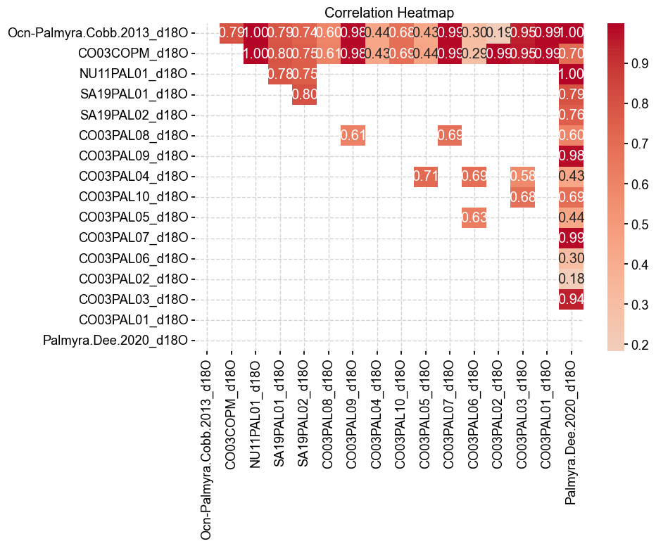
../../_images/0fa32dd6c5a34e6c184e341a3c06ea629aad4d30f0951839d5332d75da29a2db.png

Some of the correlations are high, suggesting that the small segments went into the composited records. Note that some of the correlations were not run since the segments were not overlapping and were, therefore, skipped.

Option 2: DTW#

Let’s look at the DTW method to identify duplicates.

# --- Prepare the data ----
records = {}
times = {}

for series in mgs.series_list:
    records[series.label] = series.value
    times[series.label] = series.time


# --- Main loop ---
labels = list(records.keys())
n = len(labels)
dtw_matrix = np.full((n, n), np.nan)

for i, j in itertools.combinations(range(n), 2):
    key_i, key_j = labels[i], labels[j]

    s1, s2 = clip_to_overlap(times[key_i], records[key_i],
                             times[key_j], records[key_j])

    if s1 is not None:
        path = dtw.warping_path(s1, s2)
        dist = dtw.distance(s1, s2)
        norm_dist = dist / len(path)  # Per-step normalization

        dtw_matrix[i, j] = dtw_matrix[j, i] = norm_dist

# Convert to DataFrame for visualization
dtw_df = pd.DataFrame(dtw_matrix, index=labels, columns=labels)

plt.figure(figsize=(10, 8))
sns.heatmap(dtw_df, annot=True, fmt=".2f", cmap="viridis", mask=np.isnan(dtw_df))
plt.title("DTW Distance Matrix (Clipped to Overlap)")
plt.tight_layout()
plt.show()

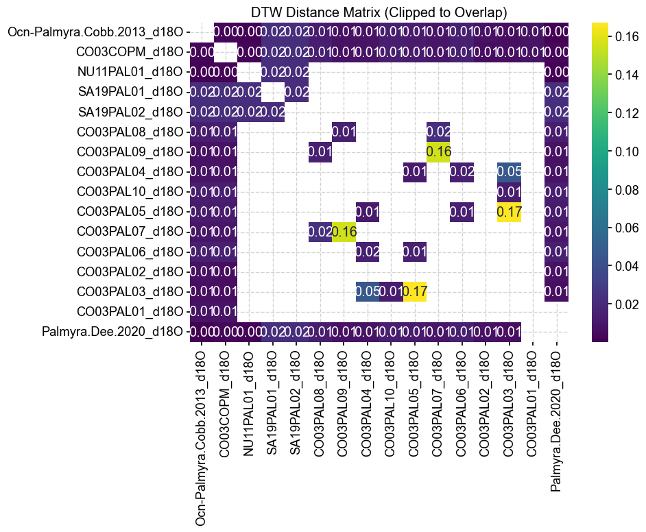
../../_images/4ed09d165fbe918929567d228e1d127605956f527dab87b451273c7511f65188.png

The DTW method largely confirms what we have seen from the correlations in terms of duplicates. However, note that the DTW method indicates that the records from OCN-Palmyra.Cobb.2013 and CO03COPM have a correlation of 0.79 but a DTW of 0. The DTW would essentially indicate that they are in fact the same records but the correlation is less than 0.8. This is due to the interpolation needed to calculate correlation over the 14th century, highlighting the need to run DTW for records with larger gaps. We will use the insights gained here to clean the database in the next section of this notebook. For now, let’s add the Dee et al. (2020) record to the database:

df_raw = pd.concat([df_raw, df_palm_filt], ignore_index=True)
df_raw.tail()

	dataSetName	compilationName	archiveType	geo_meanLat	geo_meanLon	geo_meanElev	paleoData_variableName	paleoData_standardName	paleoData_values	paleoData_units	...	paleoData_proxyGeneral	paleoData_seasonality	paleoData_interpName	paleoData_interpRank	TSID	time_variableName	time_standardName	time_values	time_units	distance_km
968	ZI08MAY01	CoralHydro2k	Coral	-12.6500	45.10	-2.0	SrCa	Sr/Ca	[8.947578, 8.797017, 8.784511, 8.751525, 8.778...	mmol/mol	...	None	None	None	NaN	ZI08MAY01_SrCa	year	year	[1881.6247, 1881.791367, 1881.958033, 1882.124...	yr AD	16936.585327
969	LI06FIJ01	CoralHydro2k	Coral	-16.8200	179.23	-10.0	d18O	d18O	[-4.6922, -4.6266, -4.6018, -4.5486, -4.6102, ...	permil	...	None	None	None	NaN	LI06FIJ01_d18O	year	year	[1617.5, 1618.5, 1619.5, 1620.5, 1621.5, 1622....	yr AD	3250.716202
970	SM06LKF02	CoralHydro2k	Coral	24.5600	-81.41	-4.0	d18O	d18O	[-3.85, -3.98, -4.21, -4.06, -3.97, -4.04, -3....	permil	...	None	None	None	NaN	SM06LKF02_d18O	year	year	[1960.97, 1961.03, 1961.09, 1961.15, 1961.21, ...	yr AD	8799.120973
971	SM06LKF02	CoralHydro2k	Coral	24.5600	-81.41	-4.0	SrCa	Sr/Ca	[9.225, nan, 9.195, 9.221, 9.198, 9.281, 9.319...	mmol/mol	...	None	None	None	NaN	SM06LKF02_SrCa	year	year	[1960.97, 1961.03, 1961.09, 1961.15, 1961.21, ...	yr AD	8799.120973
972	Palmyra.Dee.2020	None	Coral	5.8664	-162.12	-9.0	d18O	d18O	[-4.749, -4.672, -4.724, -4.717, -4.8947, -4.8...	permil	...	isotopic	subannual	temperature	NaN	PCU-1cce3af5639a4ec	year	year	[1146.375, 1146.4583, 1146.5417, 1146.625, 114...	yr AD	NaN

5 rows × 21 columns

Let’s drop the added columns that we put in for distance:

df_raw = df_raw.drop(columns=['distance_km'])

Data Cleaning and Pre-processing#

This section deals with cleaning and pre-processing for use with the cfr codebase. We will do so in three steps:

Step 1: Remove records that are less than 150 years. For reconstruction purposes, we need series that go back at least to 1850; many in this database do not, so we remove them to avoid disappointments later on.
Step 2: Remove duplicates. We will use an algorithm based on the data exploratory analysis we did for the specific case of the Palmyra record and generalize it.
Step 3: Filtering for records with annual to subannual resolution.

Step 1: Remove records shorter than 150 years#

For reconstruction purposes, we need series that go back at least to 1850; many in this database do not, so we remove them to avoid disappointments later on. Let’s first look at the start date of these records.

df_raw['min_time'] = df_raw['time_values'].apply(lambda x: min(x) if isinstance(x, list) and x else float('inf'))
filtered_df = df_raw[df_raw['min_time'] < 1850]
filtered_df = filtered_df.drop(columns=['min_time'])
print(filtered_df.shape)

(744, 20)

That leaves us with 744 timeseries.

Step 2: Screen for duplicates#

Based on the preliminary work we have done with the Palmyra records, we will used the following algorithm to identify duplicates:

Look for records within 10km of each other
Look at whether the variable name is the same
Calculate correlations among the records
Calculate the DTW distance among the records.
For correlations >0.8 OR DTW distance < 0.03, use the following:

a. Use the latest publication date (based on dataset name)

b. Use the longest record if the publication date is the same

Let’s have a look at the variable names present in the database to see if there are synonyms we have to deal with. Let’s make sure that we use a criteria that doesn’t have any missing values:

filtered_df.info()

<class 'pandas.core.frame.DataFrame'>
Index: 744 entries, 0 to 972
Data columns (total 20 columns):
 #   Column                  Non-Null Count  Dtype  
---  ------                  --------------  -----  
 dataSetName             744 non-null    object 
 compilationName         743 non-null    object 
 archiveType             744 non-null    object 
 geo_meanLat             744 non-null    float64
 geo_meanLon             744 non-null    float64
 geo_meanElev            737 non-null    object 
 paleoData_variableName  744 non-null    object 
 paleoData_standardName  744 non-null    object 
 paleoData_values        744 non-null    object 
 paleoData_units         336 non-null    object 
paleoData_proxy         665 non-null    object 
paleoData_proxyGeneral  501 non-null    object 
paleoData_seasonality   659 non-null    object 
paleoData_interpName    665 non-null    object 
paleoData_interpRank    12 non-null     float64
TSID                    744 non-null    object 
time_variableName       744 non-null    object 
time_standardName       744 non-null    object 
time_values             744 non-null    object 
time_units              744 non-null    object 
dtypes: float64(3), object(17)
memory usage: 122.1+ KB

From this, it seems that paleoData_standardName could work for our purposes since there are no missing values in this field and most of the names should have been standardized:

filtered_df['paleoData_standardName'].unique()

array(['d18O', 'MXD', 'density', 'ringWidth', 'temperature',
       'reflectance', 'Sr/Ca', 'iceMelt', 'd2H', 'thickness',
       'RABD660670', 'calcificationRate', 'varveThickness', 'MAR'],
      dtype=object)

The names are unique. Let’s proceed with the main loop. But first, let’s define some constants and parameters for the algorithm described above:

# --- Define some parameters ---
threshold  = 10 # Distance in km
corr_threshold = 0.8 # Corr threshold over which two records are considered the same. 
dtw_threshold = 0.03 # DTW threshold under which two records are considered the same. 

Let’s also consider writing some functions to calculate the various criteria described above:

Distance on aa sphere using the Haversine distance
Correlation among multiple timeseries using Pyleoclim
DTW amon multiple timeseries

# --- Haversine distance function in km ---
def haversine(lat1, lon1, lats2, lons2, R=6371):
    """Calculate the haversine distance between a target location and a vector of locations. 

    Args:
        lat1 (float): The target latitude
        lon1 (float): the target longitude
        lats2 (np.array or df.Series): The latitude of the locations to check against
        lons2 (np.array or df.Series): The longitude of the locations to check against
        R (int, optional): The radius of the planet in km. Defaults to 6371 for Earth.

    Returns:
        np.array: The distance between the target location and the vector of locations in km.
    """
    # Convert degrees to radians
    lat1 = np.radians(lat1)
    lon1 = np.radians(lon1)
    lats2 = np.radians(lats2)
    lons2 = np.radians(lons2)

    # Haversine formula
    dlat = lats2 - lat1
    dlon = lons2 - lon1
    
    a = np.sin(dlat / 2)**2 + np.cos(lat1) * np.cos(lats2) * np.sin(dlon / 2)**2
    c = 2 * np.arcsin(np.sqrt(a))

    return R*c


# ----- Correlation function ------

def correlation(data):
    """Calculate correlation among multiple timeseries

    Parameters
    ----------
    data: pd.DataFrame
        A pandas DataFrame containing the necessary information to create Pyleoclim.GeoSeries() objects
    
    Returns
    -------
    A DataFrame containing pairwise correlations
    """
    ds_name1 = [] # list of dataset names used as correlation basis
    ds_name2 = [] # list of dataset names used as the series to correlate against
    # Same for tsids since they are unique and we can find them again easily in the database
    tsid1 = []
    tsid2 = []
    # list to keep the correlations
    corr = []

    # Create a MultipleGeoSeries object

    ts_list = []

    for idx, row in data.iterrows():

        ts = pyleo.GeoSeries(time=row['time_values'],value=row['paleoData_values'],
                            time_name='Time',value_name=row['paleoData_standardName'],
                            time_unit=row['time_units'], value_unit=row['paleoData_units'],
                            lat = row['geo_meanLat'], lon = row['geo_meanLon'], 
                            elevation = row['geo_meanElev'], archiveType = row['archiveType'],    
                            label=row['TSID']+'+'+row['dataSetName'], verbose = False)
        ts_list.append(ts)

    for i,j in itertools.combinations(range(len(ts_list)), 2):
        ts1 = ts_list[i] #grab the first timeseries
        ts2 = ts_list[j]

        # append the names and tsids
        ds_name1.append(ts1.label.split('+')[1])
        tsid1.append(ts1.label.split('+')[0])
                
        ds_name2.append(ts2.label.split('+')[1])
        tsid2.append(ts2.label.split('+')[0])

        # calculate the correlation
        corr_res = ts1.correlation(ts2, method = 'built-in')

        # Store the information
        corr.append(corr_res.r)
    
    # Step 3: Summarize results

    return pd.DataFrame({'dataSetName1': ds_name1,
                         'dataSetName2': ds_name2,
                         'TSID1': tsid1,
                         'TSID2': tsid2,
                        'correlation': corr}) 


# ------ DTW function


def dtw_pair(data):
    """Calculates the DTW betwen the records in the dataframe

    Args:
        data (pd.DataFrame): A pandas DataFrame containing the necessary information to create Pyleoclim.GeoSeries() objects

    Returns:
        pd.DataFrame: A DataFrame containing pairwise DTW
    """

    ### Helper function
    
    def clip_to_overlap(time1, series1, time2, series2, min_overlap=5):
        """Helper function to clip the series to common overlap. Note we do  not need to interpolate for DTW, just make sure that the time is overlapping

        Args:
            time1 (np.array): Time vector for Series 1
            series1 (np.array): Value vector for Series 1
            time2 (np.array): Time vector for Series 2
            series2 (np.array): Value vector for Series 2
            min_overlap (int, optional): Minimum number of pointe to even attempt the computation. Defaults to 5.

        Returns:
            np.array, np.array: The zscore of the values for the time of overlap.  
        """
        # Make sure things are sorted and have no NaNs
        valid1 = (~np.isnan(time1)) & (~np.isnan(series1))
        time1 = time1[valid1]
        series1 = series1[valid1]

        valid2 = (~np.isnan(time2)) & (~np.isnan(series2))
        time2 = time2[valid2]
        series2 = series2[valid2]

        # Return early if either series is now empty
        if len(time1) == 0 or len(time2) == 0:
            return None, None


        sort_idx1 = np.argsort(time1)
        time1_sorted = time1[sort_idx1]
        series1_sorted = series1[sort_idx1]

        sort_idx2 = np.argsort(time2)
        time2_sorted = time2[sort_idx2]
        series2_sorted = series2[sort_idx2]

        # Determine overlapping interval
        start = max(time1_sorted[0], time2_sorted[0])
        end = min(time1_sorted[-1], time2_sorted[-1])

        # Apply mask
        mask1 = (time1_sorted >= start) & (time1_sorted <= end)
        mask2 = (time2_sorted >= start) & (time2_sorted <= end)

        if np.sum(mask1) < min_overlap or np.sum(mask2) < min_overlap:
            return None, None # Not enough overlapping points

        clipped1 = series1_sorted[mask1]
        clipped2 = series2_sorted[mask2]

        # Avoid division by zero if std = 0
        if np.std(clipped1) == 0 or np.std(clipped2) == 0:
            return None, None

        return zscore(clipped1), zscore(clipped2)
   
    ### Main function 

    ds_name1 = [] # list of dataset names used as correlation basis
    ds_name2 = [] # list of dataset names used as the series to correlate against
    # Same for tsids since they are unique and we can find them again easily in the database
    tsid1 = []
    tsid2 = []
    # list to keep the DTW
    dtw_list = []

    for idx1, idx2 in itertools.combinations(data.index, 2):
        row1 = data.loc[idx1] #grab the first record
        row2 = data.loc[idx2] #grab the second record

        ds_name1.append(row1['dataSetName'])
        ds_name2.append(row2['dataSetName'])
        tsid1.append(row1['TSID'])
        tsid2.append(row2['TSID'])

        s1, s2 = clip_to_overlap(np.array(row1['time_values']), np.array(row1['paleoData_values']),
                                 np.array(row2['time_values']), np.array(row2['paleoData_values']))
        

        if s1 is not None:
            path = dtw.warping_path(s1, s2)
            dist = dtw.distance(s1, s2)
            dtw_list.append(dist / len(path))  # Per-step normalization
        else:
            dtw_list.append(np.nan)

    df= pd.DataFrame({'dataSetName1': ds_name1,
                       'dataSetName2': ds_name2,
                       'TSID1': tsid1,
                       'TSID2': tsid2,
                       'dtw': dtw_list})
        
    return df
    

df_list = [] # Containers for the list of DataFrames with spurious correlations
tsids = [] #to keep track of the tsids that have already been checked against the distance criteria

#make a copy of the dataframe as we need to modify it for this loop
df_copy = filtered_df.copy()

for idx, row in df_copy.iterrows():

    # Check that we haven't already looked at the record in the context of another distance search

    if row['TSID'] in tsids:
        continue #go to the next row

    # ---- Criteria 1: Distance -----
    # Target location
    lat1, lon1 = row['geo_meanLat'], row['geo_meanLon']
    distance_km = haversine(lat1,lon1,df_copy['geo_meanLat'],df_copy['geo_meanLon'])

    # Add distance column
    df_copy['distance_km'] = distance_km

    # Filter to only rows within a threshold
    df_distance = df_copy[df_copy['distance_km'] <= threshold].reset_index(drop=True)

    # Store the TSIDs so we don't run this multiple times
    tsids.extend(df_distance['TSID'].to_list())

    # If there is only one entry (the original one, go to the next row)
    if len(df_distance)<=1:
        continue

    # ---- Criteria 2: Variable Name ------

    var_unique = df_distance['paleoData_standardName'].unique()

    for var in var_unique:
        df_var_filt = df_distance[df_distance['paleoData_standardName'] == var].reset_index(drop=True)
        
        if len(df_var_filt) >1:

    # ----- Criteria 3: Correlation -------
            corr_df = correlation(df_var_filt)
    
    # ------ Criteria 4: DTW --------
            dtw_df = dtw_pair(df_var_filt)
        
            #put the results together
            common_cols = ['dataSetName1', 'dataSetName1', 'TSID1','TSID2']

            df_combined = pd.merge(corr_df, dtw_df, on=common_cols)
            df_res = df_combined[(df_combined['correlation'] > corr_threshold) | (df_combined['dtw'] < dtw_threshold)]

            if not df_res.empty:
                df_list.append(df_res)

Let’s see how many similar records we have:

len(df_list)

Let’s have a look at each records with duplicated and create a log (human in the loop) of why records were removed from the database.

⚠️ Warning

The following cell produces a widget that allows you to go through each of the similar records and to keep/remove records. If you do so, you will change the nature of the database.

❗ DO NOT RUN THIS CELL UNLESS YOU WANT TO CLEAN THE DATABASE YOURSELF. NOT RECOMMENDED!!!!!! Skip to the last section to load the cleaned database directly.

from IPython.display import display, clear_output, Markdown import ipywidgets as widgets # Storage flagged_records = [] group_notes = [] df_copy = filtered_df.copy() index_tracker = {'i': 0} def run_iteration(i): clear_output(wait=True) # Final screen if i >= len(df_list): print("✅ Review complete!") if flagged_records: print("\n🚩 Flagged TSIDs:") display(pd.DataFrame(flagged_records)) else: print("\n🚩 No TSIDs were flagged.") if group_notes and any(n['Note'].strip() for n in group_notes): print("\n📝 Notes from each group:") markdown_notes = "\n\n".join( [ f"### Iteration {note['Group'] + 1}\n" f"```\n{note['Note']}\n```" for note in group_notes if note['Note'].strip() ] ) display(Markdown(markdown_notes)) else: print("\n📝 No group notes were entered.") # Final Done button done_button = widgets.Button(description="Done", button_style='success') def on_done_clicked(b): clear_output(wait=True) print("🎉 Done! You may now export your results.") done_button.on_click(on_done_clicked) display(done_button) return # Begin reviewing group i df = df_list[i] print(f"--- Reviewing DataFrame {i+1}/{len(df_list)} ---") valid_ids = pd.concat([df['TSID1'], df['TSID2']]).unique() df_lookup = df_copy[df_copy['TSID'].isin(valid_ids)] display(df_lookup) # Plot time series ts_list = [] for _, row in df_lookup.iterrows(): ts = pyleo.GeoSeries( time=row['time_values'], value=row['paleoData_values'], time_name='Time', value_name=row['paleoData_standardName'], time_unit=row['time_units'], value_unit=row['paleoData_units'], lat=row['geo_meanLat'], lon=row['geo_meanLon'], elevation=row['geo_meanElev'], archiveType=row['archiveType'], label=row['TSID'] + '+' + row['dataSetName'], verbose=False ) ts_list.append(ts) if ts_list: mgs = pyleo.MultipleGeoSeries(ts_list) fig, ax = mgs.stackplot() fig.show() else: print("No valid time series to plot.") # Create widgets for TSIDs tsid_widgets = [] for tsid in valid_ids: toggle = widgets.RadioButtons( options=['Keep', 'Remove'], value='Keep', description=f'{tsid}:', layout=widgets.Layout(width='40%') ) tsid_widgets.append((tsid, toggle)) toggle_box = widgets.VBox([w[1] for w in tsid_widgets]) # Shared note box (pre-filled) note_template = "Records from different samples. Not true duplicates." note_box = widgets.Textarea( value=note_template, layout=widgets.Layout(width='100%', height='60px') ) # Buttons next_button = widgets.Button(description="Next", button_style='success') back_button = widgets.Button(description="Back", button_style='warning') quit_button = widgets.Button(description="Quit", button_style='danger') button_box = widgets.HBox([next_button, back_button, quit_button]) # --- Button callbacks --- def on_next_clicked(b): note = note_box.value.strip() # Remove prior flags and note for this group group_notes[:] = [n for n in group_notes if n['Group'] != i] flagged_records[:] = [r for r in flagged_records if r['TSID'] not in valid_ids] # Save new notes and flags group_notes.append({'Group': i, 'Note': note}) for tsid, toggle in tsid_widgets: if toggle.value == 'Remove': flagged_records.append({'TSID': tsid, 'Note': note}) index_tracker['i'] += 1 run_iteration(index_tracker['i']) def on_back_clicked(b): if index_tracker['i'] > 0: index_tracker['i'] -= 1 run_iteration(index_tracker['i']) else: print("You're already at the first group.") def on_quit_clicked(b): clear_output(wait=True) print("⚠️ Quit early.") if flagged_records: print("\n🚩 Flagged TSIDs:") display(pd.DataFrame(flagged_records)) if group_notes and any(n['Note'].strip() for n in group_notes): print("\n📝 Notes from each group:") markdown_notes = "\n\n".join( [ f"### Iteration {note['Group'] + 1}\n" f"```\n{note['Note']}\n```" for note in group_notes if note['Note'].strip() ] ) display(Markdown(markdown_notes)) else: print("\n📝 No group notes were entered.") # Hook up buttons next_button.on_click(on_next_clicked) back_button.on_click(on_back_clicked) quit_button.on_click(on_quit_clicked) # Display UI display(button_box, toggle_box, note_box) # Start the interactive loop run_iteration(index_tracker['i'])

TSID Note

0 Ocean2kHR_142_iso2k Ocean2kHR_142_iso2k is a duplicate of Ocean2kH...

1 Ocean2kHR_156_iso2k Ocean2kHR_142_iso2k is a duplicate of Ocean2kH...

2 Ocean2kHR_157_iso2k Ocean2kHR_142_iso2k is a duplicate of Ocean2kH...

3 LI00RAR01_d18O Same records. Keeping 147.

4 LI00RAR01_SrCa Same record. Keeping 149

5 Ocean2kHR_006_iso2k Same records, keeping Ocean2kHR_006 from PAGES2k

6 CH03LOM01_d18O Same records, keeping Ocean2kHR_006 from PAGES2k

7 Ocean2kHR_019_iso2k Same record. Keeping Ocean2kHR_019

8 FE18RUS01_d18O Same record. Keeping Ocean2kHR_019

9 CA07FLI01_SrCa Records from different samples. Not true dupli...

10 Ocean2kHR_193_iso2k Same record. Keeping Ocean2kHR_193

11 CA07FLI01_d18O Same record. Keeping Ocean2kHR_193

12 Ocean2kHR_026_iso2k Two records but duplicates. Keeping Ocean2kHR_...

13 KU99HOU01_d18O Two records but duplicates. Keeping Ocean2kHR_...

14 ZI14HOU01_d18O Two records but duplicates. Keeping Ocean2kHR_...

15 ZI14HOU01_SrCa Two records. Keeping Ocean2kHR 027 and 025

16 Ocean2kHR_133_iso2k Same record across all compilations. Keeping O...

17 QU96ESV01_d18O Same record across all compilations. Keeping O...

18 Ocean2kHR_183_iso2k Same record across all three compilations. Kee...

19 OS14UCP01_d18O Same record across all three compilations. Kee...

20 Ocean2kHR_166_iso2k Same record across all three compilations. Kee...

21 AS05GUA01_d18O Same record across all three compilations. Kee...

22 KI08PAR01_d18O Same record from two different compilations. K...

23 Ocean2kHR_173_iso2k Same record from three different compilations....

24 DU94URV01_d18O Same record from three different compilations....

25 Ocean2kHR_001_iso2k Same record from three different compilations....

26 CO00MAL01_d18O Same record from three different compilations....

27 DR99ABR01_d18O Same record from two different compilations. K...

28 Ocean2kHR_094_iso2k Same record from two different compilations. K...

29 Ocean2kHR_007_iso2k Same record from three compilations (note that...

30 DA06MAF02_d18O Same record from three compilations (note that...

31 Ocean2kHR_177_iso2k Same record from three different compilations....

32 UR00MAI01_d18O Same record from three different compilations....

33 SAm_035_iso2k Same record from two different compilations. K...

34 Ocean2kHR_139 Palmyra record!!!! Keeping PCU-1cce3af5639a4ec...

35 Ocean2kHR_139_iso2k Palmyra record!!!! Keeping PCU-1cce3af5639a4ec...

36 CO03PAL08_d18O Palmyra record!!!! Keeping PCU-1cce3af5639a4ec...

37 CO03PAL09_d18O Palmyra record!!!! Keeping PCU-1cce3af5639a4ec...

38 CO03PAL04_d18O Palmyra record!!!! Keeping PCU-1cce3af5639a4ec...

39 CO03PAL10_d18O Palmyra record!!!! Keeping PCU-1cce3af5639a4ec...

40 CO03PAL05_d18O Palmyra record!!!! Keeping PCU-1cce3af5639a4ec...

41 CO03PAL07_d18O Palmyra record!!!! Keeping PCU-1cce3af5639a4ec...

42 CO03PAL06_d18O Palmyra record!!!! Keeping PCU-1cce3af5639a4ec...

43 CO03PAL02_d18O Palmyra record!!!! Keeping PCU-1cce3af5639a4ec...

44 CO03PAL03_d18O Palmyra record!!!! Keeping PCU-1cce3af5639a4ec...

45 CO03PAL01_d18O Palmyra record!!!! Keeping PCU-1cce3af5639a4ec...

46 Ocean2kHR_020_iso2k Same record from different compilations. Keepi...

47 ZI04IFR01_d18O Same record from different compilations. Keepi...

48 DE12ANC01_SrCa Same record from two different compilations. K...

49 WE09ARR01_d18O Same record from two different compilations. K...

50 WE09ARR01_SrCa Same record from two different compilations. K...

51 Ocean2kHR_013_iso2k Same record from two different compilations. K...

52 Ocean2kHR_126_iso2k Same record from different compilations. Keepi...

53 Ocean2kHR_105_iso2k Same reocords. Keeping Ocean2kHR 102 and 105 a...

54 Ocean2kHR_102_iso2k Same reocords. Keeping Ocean2kHR 102 and 105 a...

55 Ocean2kHR_154_iso2k Same record from different compilation. Keepin...

56 GO12SBV01_d18O Same record from different compilation. Keepin...

57 WU13TON01_SrCa Same record from different compilations. Keepi...

58 Ocean2kHR_138_iso2k Same record from different compilations. Keepi...

59 LI94SEC01_d18O Same record from different compilations. Keepi...

Iteration 1

Records from different samples. Not true duplicates.

Iteration 2

Records from different samples. Not true duplicates.

Iteration 3

Records from different samples. Not true duplicates.

Iteration 4

Records from different samples. Not true duplicates.

Iteration 5

Records from different samples. Not true duplicates.

Iteration 6

Records from different samples. Not true duplicates.

Iteration 7

Records from different samples. Not true duplicates.

Iteration 8

Records from different samples. Not true duplicates.

Iteration 9

Ocean2kHR_142_iso2k is a duplicate of Ocean2kHR_142 deom most likely PAGES2k. Removing iso2k record. Same with 156 and 157

Iteration 10

From publications info in GraphDB. Different records.

Iteration 11

Same records. Keeping 147.

Iteration 12

Same record. Keeping 149

Iteration 13

Same records, keeping Ocean2kHR_006 from PAGES2k

Iteration 14

Same record. Keeping Ocean2kHR_019

Iteration 15

Records from different samples. Not true duplicates.

Iteration 16

Records from different samples. Not true duplicates.

Iteration 17

Same record. Keeping Ocean2kHR_193

Iteration 18

Two records but duplicates. Keeping Ocean2kHR_023 and 026.

Iteration 19

Two records. Keeping Ocean2kHR 027 and 025

Iteration 20

Same record across all compilations. Keeping Ocean2kHR_133

Iteration 21

Records from different samples. Not true duplicates.

Iteration 22

Same record across all three compilations. Keeping Ocean2kHR_183

Iteration 23

Same record across all three compilations. Keeping Ocean2kHR166

Iteration 24

Records from different samples. Not true duplicates.

Iteration 25

Records from different samples. Not true duplicates.

Iteration 26

Records from different samples. Not true duplicates.

Iteration 27

Records from different samples. Not true duplicates.

Iteration 28

Records from different samples. Not true duplicates.

Iteration 29

Records from different samples. Not true duplicates.

Iteration 30

Same record from two different compilations. Keeping Ocean2kHR_099

Iteration 31

Same record from two different compilations. Keeping Ocean2HR_100

Iteration 32

Records from different samples. Not true duplicates.

Iteration 33

Records from different samples. Not true duplicates.

Iteration 34

Same record from three different compilations. Keeping Ocean2kHR_173

Iteration 35

Records from different samples. Not true duplicates.

Iteration 36

Same record from three different compilations. Keeping Ocean2kHR_001

Iteration 37

Records from different samples. Not true duplicates.

Iteration 38

Records from different samples. Not true duplicates.

Iteration 39

Records from different samples. Not true duplicates.

Iteration 40

Same record from two different compilations. Keeping Ocean2kHR_167

Iteration 41

Same record from two different compilations. Keeping Ocean2kHR_094

Iteration 42

Same record from three compilations (note that it's most likely from two different coral head which CoralHydro2k archived in different dataset). Keeping Ocean2kHR_007

Iteration 43

Records from different samples. Not true duplicates.

Iteration 44

Records from different samples. Not true duplicates.

Iteration 45

Records from different samples. Not true duplicates.

Iteration 46

Records from different samples. Not true duplicates.

Iteration 47

Same record from three different compilations. Keeping Ocean2kHR_177

Iteration 48

Records from different samples. Not true duplicates.

Iteration 49

Same record from two different compilations. Keeping SAm_035

Iteration 50

Records from different samples. Not true duplicates.

Iteration 51

Records from different samples. Not true duplicates.

Iteration 52

Records from different samples. Not true duplicates.

Iteration 53

Palmyra record!!!! Keeping PCU-1cce3af5639a4ec from Dee et al. (2020)

Iteration 54

Records from different samples. Not true duplicates.

Iteration 55

Records from different samples. Not true duplicates.

Iteration 56

Records from different samples. Not true duplicates.

Iteration 57

Records from different samples. Not true duplicates.

Iteration 58

Records from different samples. Not true duplicates.

Iteration 59

Records from different samples. Not true duplicates.

Iteration 60

Records from different samples. Not true duplicates.

Iteration 61

Records from different samples. Not true duplicates.

Iteration 62

Same record from different compilations. Keeping Ocean2kHR_020

Iteration 63

Records from different samples. Not true duplicates.

Iteration 64

Records from different samples. Not true duplicates.

Iteration 65

Records from different samples. Not true duplicates.

Iteration 66

Same record from two different compilations. Keeping Ocean2kHR_134

Iteration 67

Records from different samples. Not true duplicates.

Iteration 68

Records from different samples. Not true duplicates.

Iteration 69

Records from different samples. Not true duplicates.

Iteration 70

Records from different samples. Not true duplicates.

Iteration 71

Same record from two different compilations. Keeping Ocean2kHR_190

Iteration 72

Same record from two different compilations. Keeping Ocean2kHR_191

Iteration 73

Records from different samples. Not true duplicates.

Iteration 74

Records from different samples. Not true duplicates.

Iteration 75

Same record from two different compilations. Keeping Ocean2kHR_013

Iteration 76

Records from different samples. Not true duplicates.

Iteration 77

Records from different samples. Not true duplicates.

Iteration 78

Records from different samples. Not true duplicates.

Iteration 79

Records from different samples. Not true duplicates.

Iteration 80

Same record from different compilations. Keeping Ocean2kHR_126

Iteration 81

Same reocords. Keeping Ocean2kHR 102 and 105 as well as DR00NBB01, which seems to be unique

Iteration 82

Records from different samples. Not true duplicates.

Iteration 83

Same record from different compilation. Keeping Ocean2kHR_154

Iteration 84

Same record from different compilations. Keeping Ocean2kHR_159

Iteration 85

Records from different samples. Not true duplicates.

Iteration 86

Same record from different compilations. Keeping Ocean2kHR_138

Iteration 87

Records from different samples. Not true duplicates.

Iteration 88

Records from different samples. Not true duplicates.

Iteration 89

Records from different samples. Not true duplicates.

# Save flagged TSIDs and notes df_flags = pd.DataFrame(flagged_records) df_flags.to_csv("./data/flagged_tsids_with_notes.csv", index=False) df_notes = pd.DataFrame(group_notes) df_notes.to_csv("./data/group_notes.csv", index=False) # Cleaned dataset df_cleaned = df_copy[~df_copy['TSID'].isin(df_flags['TSID'])]

# save the file df_cleaned.to_pickle("./data/cleaned_timeseries.pkl")

Building the cfr.ProxyDataBase#

Reopen the file:

df_cleaned = pd.read_pickle("./data/cleaned_timeseries.pkl") df_cleaned.head()

dataSetName compilationName archiveType geo_meanLat geo_meanLon geo_meanElev paleoData_variableName paleoData_standardName paleoData_values paleoData_units paleoData_proxy paleoData_proxyGeneral paleoData_seasonality paleoData_interpName paleoData_interpRank TSID time_variableName time_standardName time_values time_units

0 Ant-WDC05A.Steig.2013 Pages2kTemperature Glacier ice -79.46 -112.09 1806.0 d18O d18O [-33.32873325, -35.6732, -33.1574, -34.2854, -... permil d18O None Annual temperature NaN Ant_030 year year [2005, 2004, 2003, 2002, 2001, 2000, 1999, 199... yr AD

1 NAm-MtLemon.Briffa.2002 Pages2kTemperature Wood 32.50 -110.80 2700.0 MXD MXD [0.968, 0.962, 1.013, 0.95, 1.008, 0.952, 1.02... None maximum latewood density dendrophysical Summer temperature NaN NAm_568 year year [1568, 1569, 1570, 1571, 1572, 1573, 1574, 157... yr AD

2 Arc-Arjeplog.Bjorklund.2014 Pages2kTemperature Wood 66.30 18.20 800.0 density density [-0.829089212152348, -0.733882889924006, -0.89... None maximum latewood density dendrophysical Jun-Aug temperature NaN Arc_060 year year [1200, 1201, 1202, 1203, 1204, 1205, 1206, 120... yr AD

3 Asi-CHIN019.Li.2010 Pages2kTemperature Wood 29.15 99.93 2150.0 ringWidth ringWidth [1.465, 1.327, 1.202, 0.757, 1.094, 1.006, 1.2... None ring width dendrophysical Annual temperature NaN Asia_041 year year [1509, 1510, 1511, 1512, 1513, 1514, 1515, 151... yr AD

4 NAm-Landslide.Luckman.2006 Pages2kTemperature Wood 60.20 -138.50 800.0 ringWidth ringWidth [1.123, 0.841, 0.863, 1.209, 1.139, 1.056, 0.8... None ring width dendrophysical Summer temperature NaN NAm_1876 year year [913, 914, 915, 916, 917, 918, 919, 920, 921, ... yr AD

Adding ptype and seasonality info#

LiPD files contain seasonality (in months or phrases) and the necessary information to create a cfr ‘ptype’. The ‘ptype’ is simply the proxy archive and variable name, for example d18O of coral would be coral.d18O. The seasonality on the other hand, requires some conversion between month to the numerical list format that cfr accepts. For example, for a growing season of June, July, August, the cfr seasonality will be [6,7,8]. In the following two functions convert_seasonality and create_ptype, we can get the original dataFrame columns into the format we need for assimilation.

def convert_seasonality(seasonality_str, latitude = None): """ Convert LiPD seasonality strings to CFR month lists CFR expects lists like [6,7,8] for JJA, [12,1,2] for DJF, etc. Args: seasonality_str: String representation of seasonality from LiPD Returns: list: List of month integers, or list(range(1,13)) for annual/None """ # Default to annual for None/NaN if pd.isna(seasonality_str) or seasonality_str == '' or seasonality_str is None: return list(range(1, 13)) seasonality_str = str(seasonality_str).strip() # Hemisphere-aware mapping for Summer/Winter and Growing season if seasonality_str in ['Summer', 'Winter'] and latitude is not None: if latitude > 0: # NH if seasonality_str == 'Summer': return [6, 7, 8] # JJA elif seasonality_str == 'Winter': return [12, 1, 2] # DJF elif latitude < 0: # SH if seasonality_str == 'Summer': return [12, 1, 2] # DJF in NH = Summer in SH elif seasonality_str == 'Winter': return [6, 7, 8] # JJA in NH = Winter in SH if seasonality_str in ['Growing Season'] and latitude is not None: if latitude > 0: # NH return [4, 5, 6, 7, 8, 9] # Apr-Sept else: # SH return [10, 11, 12, 1, 2, 3] # Oct-Mar # Exact mapping for your specific seasonality patterns seasonality_map = { 'Annual': list(range(1, 13)), 'Jun-Aug': [6, 7, 8], 'Nov-Feb': [11, 12, 1, 2], 'May-Apr': [5, 6, 7, 8, 9, 10, 11, 12, 1, 2, 3, 4], # May to next April 'Jun-Jul': [6, 7], 'Mar-May': [3, 4, 5], 'subannual': list(range(1, 13)), # Default to annual?? 'Sep-Apr': [9, 10, 11, 12, 1, 2, 3, 4], 'Jul': [7], 'Dec-Feb': [12, 1, 2], 'Apr': [4], 'Jul-Jun': [7, 8, 9, 10, 11, 12, 1, 2, 3, 4, 5, 6], # Jul to next June 'Sep-Nov': [9, 10, 11], 'Nov-Oct': [11, 12, 1, 2, 3, 4, 5, 6, 7, 8, 9, 10], # Nov to next Oct 'Apr-Jul': [4, 5, 6, 7], 'Jul-Sep': [7, 8, 9], 'Oct-Apr': [10, 11, 12, 1, 2, 3, 4], 'Nov-Apr': [11, 12, 1, 2, 3, 4], 'Apr-Sep': [4, 5, 6, 7, 8, 9], 'Dec-Mar': [12, 1, 2, 3], 'Aug-Jul': [8, 9, 10, 11, 12, 1, 2, 3, 4, 5, 6, 7], # Aug to next July 'Jun-Sep': [6, 7, 8, 9], 'Sep-Aug': [9, 10, 11, 12, 1, 2, 3, 4, 5, 6, 7, 8], # Sep to next Aug 'Mar-Aug': [3, 4, 5, 6, 7, 8], 'Jun': [6], 'May-Sep': [5, 6, 7, 8, 9], 'Feb-Aug': [2, 3, 4, 5, 6, 7, 8], 'Jul-Dec': [7, 8, 9, 10, 11, 12], 'Mar-Oct': [3, 4, 5, 6, 7, 8, 9, 10], 'May-Jul': [5, 6, 7], 'Jan-Mar': [1, 2, 3], 'Apr-Jun': [4, 5, 6], } # Direct lookup if seasonality_str in seasonality_map: return seasonality_map[seasonality_str] # If no pattern matches, default to annual print(f"Warning: Could not parse seasonality '{seasonality_str}', defaulting to annual") return list(range(1, 13))

def create_ptype(archive_type, proxy_standard_name): """ Determine CFR proxy type from LiPD archive and proxy information Args: archive_type: LiPD archiveType proxy_standard_name: LiPD paleoData_standardName Returns: str: CFR-compatible proxy type string """ archive = str(archive_type).lower() if pd.notna(archive_type) else 'unknown' proxy = str(proxy_standard_name).lower() if pd.notna(proxy_standard_name) else 'unknown' if 'wood' in archive or 'tree' in archive: if 'ring width' in proxy or 'trw' in proxy: return 'tree.TRW' elif 'density' in proxy or 'mxd' in proxy: return 'tree.MXD' else: return 'tree.TRW' elif 'coral' in archive: if 'd18o' in proxy: return 'coral.d18O' elif 'sr/ca' in proxy: return 'coral.SrCa' elif 'calcification' in proxy: return 'coral.calc' else: return 'coral.d18O' elif 'ice' in archive: if 'dD' in proxy or 'd2H' in proxy: return 'ice.dD' elif 'melt' in proxy: return 'ice.melt' else: return 'ice.d18O' elif 'lake' in archive: if 'varve thickness' in proxy: return 'lake.varve_thickness' elif 'varve' in proxy and 'thickness' not in proxy: return 'lake.varve_property' elif 'chironomid' in proxy: return 'lake.chironomid' elif 'midge' in proxy: return 'lake.midge' elif 'reflectance' in proxy: return 'lake.reflectance' elif 'bsi' in proxy: return 'lake.BSi' elif 'accumulation' in proxy: return 'lake.accumulation' else: return 'lake.other' elif 'marine' in archive: if 'alkenone' in proxy: return 'marine.alkenone' elif 'mg/ca' in proxy: return 'marine.MgCa' else: return 'marine.other' elif 'documents' in archive: return 'documents' elif 'borehole' in archive: return 'borehole' elif 'speleothem' in archive: return 'speleothem.d18O' elif 'sclerosponge' in archive: return 'sclerosponge.d18O' elif 'bivalve' in archive: return 'bivalve.d18O' else: return 'hybrid'

Paleodata can sometimes be published in descending time order rather than ascending. This creates a problem for us since the cfr.ProxyRecord.dt or the median time difference between data points will register the dt < 0 when the time values are in descending order. To prevent this issue before creating any proxy databases, we will use flip_df to reverse the time values that are incorrect to keep it consistent.

def flip_df(df): """ Fix reverse time series in DataFrame """ df_fixed = df.copy() fixed_count = 0 for idx, row in df_fixed.iterrows(): time_values = np.array(row['time_values']) paleo_values = np.array(row['paleoData_values']) if len(time_values) > 1: # Check if time is descending (reverse) if time_values[0] > time_values[-1]: # Flip both arrays df_fixed.at[idx, 'time_values'] = time_values[::-1] df_fixed.at[idx, 'paleoData_values'] = paleo_values[::-1] fixed_count += 1 print(f"Fixed {fixed_count} reverse time series in DataFrame") return df_fixed

# apply the seasonality into new column df_cleaned['cfr_seasonality'] = df_cleaned.apply(lambda row: convert_seasonality(row['paleoData_seasonality'], row['geo_meanLat']), axis=1 )

# apply ptype conversion into new column df_cleaned['cfr_ptype'] = df_cleaned.apply( lambda row: create_ptype(row['archiveType'], row['paleoData_standardName']), axis=1 )

# Create new dataframe with correctly reversed time/data values df_cleaned_flip = flip_df(df_cleaned)

Fixed 173 reverse time series in DataFrame

cfr.ProxyDatabase object takes in very specific parameters such as latitude, longitude, elevation, ptype, seasonality, and of course the time and data value. All of this is provided in the dataFrame, so create_pdb will seamlessly convert our necessary df columns into a cfr.Proxydatabase with all necessary data to be able to work in a data assimilation workflow.

def create_pdb(df): """ Create CFR ProxyDatabase from DataFrame that already has cfr_seasonality and cfr_ptype columns Args: df: DataFrame with cfr_seasonality and cfr_ptype columns Returns: cfr.ProxyDatabase: Ready-to-use CFR ProxyDatabase with seasonality """ print("Creating CFR ProxyDatabase from enhanced DataFrame...") records_list = [] skipped_records = 0 for idx, row in df.iterrows(): if idx % 100 == 0: print(f" Processing {idx}/{len(df)}...") try: # Get the complete time and value arrays directly time_values = np.array(row['time_values']) paleo_values = np.array(row['paleoData_values']) # Basic validation to make sure lengths match if len(time_values) != len(paleo_values) or len(time_values) == 0: skipped_records += 1 continue # Remove any NaN values valid_mask = ~(np.isnan(time_values) | np.isnan(paleo_values)) time_values = time_values[valid_mask] paleo_values = paleo_values[valid_mask] if len(time_values) == 0: skipped_records += 1 continue # Basic info (LiPD's tsid = cfr's pid) dataset_name = str(row['dataSetName']) if pd.notna(row['dataSetName']) else f"Dataset_{idx}" tsid = str(row['TSID']) if pd.notna(row['TSID']) else f"TS_{idx}" # Location lat = float(row['geo_meanLat']) if pd.notna(row['geo_meanLat']) else 0.0 lon = float(row['geo_meanLon']) if pd.notna(row['geo_meanLon']) else 0.0 # Handle elevation elev = 0.0 if pd.notna(row['geo_meanElev']): try: elev_val = row['geo_meanElev'] if str(elev_val).lower() not in ['na', 'nan', 'none', '']: elev = float(elev_val) except (ValueError, TypeError): elev = 0.0 # Use the pre-computed CFR columns seasonality = row['cfr_seasonality'] ptype = row['cfr_ptype'] # Optional metadata value_name = str(row['paleoData_variableName']) if pd.notna(row['paleoData_variableName']) else None value_unit = str(row['paleoData_units']) if pd.notna(row['paleoData_units']) else None # Create ProxyRecord directly record = cfr.ProxyRecord( pid=tsid, time=time_values, value=paleo_values, lat=lat, lon=lon, elev=elev, ptype=ptype, seasonality=seasonality, value_name=value_name, value_unit=value_unit ) records_list.append(record) except Exception as e: print(f" Error processing record {idx}: {e}") skipped_records += 1 continue # Create empty ProxyDatabase proxy_db = cfr.ProxyDatabase() for record in records_list: proxy_db += record print(f"Created CFR ProxyDatabase with {proxy_db.nrec} records") if skipped_records > 0: print(f" Skipped {skipped_records} records due to data issues") return proxy_db

Once our functions are created to go from a dataFrame into a ProxyDatabase, we will branch off into two options for the data assimilation step.

Option 1: Filter without interpolation

Create cfr.ProxyDatabase -> filter by dt <= 1 (annual + subannual only) -> save as ‘pdb_w_seasonality_annual.pkl’

Option 2: Filter with interpolation

For records with dt <= 5, interpolate to annual then refilter.

Create cfr.ProxyDatabase -> pyleo.interp -> filter by dt <=1 -> save as ‘pdb_wseasonality_interp.pkl’

Quick debug before saving ProxyDatabases#

The main thing we want to make sure here is that seasonality is preserved when we convert from a pandas Dataframe to cfr.ProxyDatabase and then to a pickle file. Here we run a quick check just to make sure the important information is saved for all the records.

print(f"\n" + "="*50) print(" >> Converting to CFR ProxyDatabase...") try: unfiltered_pdb = create_pdb(df_cleaned_flip) print(f"SUCCESS: ProxyDatabase created with {unfiltered_pdb.nrec} records") print("Proxy types:", unfiltered_pdb.type_dict) # Verify seasonality is preserved print(f"\nSeasonality verification:") seasonality_preserved = 0 for pid, record in unfiltered_pdb.records.items(): if record.seasonality is not None: seasonality_preserved += 1 print(f"Records with seasonality: {seasonality_preserved}/{unfiltered_pdb.nrec}") # Show a sample record sample_pid = list(unfiltered_pdb.records.keys())[0] sample_record = unfiltered_pdb.records[sample_pid] print(f"\nSample CFR ProxyRecord:") print(f" PID: {sample_record.pid}") print(f" Type: {sample_record.ptype}") print(f" Seasonality: {sample_record.seasonality}") print(f" Time points: {len(sample_record.time)}") print(f" Location: ({sample_record.lat:.2f}, {sample_record.lon:.2f})") except Exception as e: print(f"ERROR creating CFR ProxyDatabase: {e}") import traceback traceback.print_exc()

================================================== >> Converting to CFR ProxyDatabase... Creating CFR ProxyDatabase from enhanced DataFrame... Processing 0/684... Processing 100/684... Processing 200/684... Processing 300/684... Processing 400/684... Processing 500/684... Processing 600/684... Created CFR ProxyDatabase with 684 records SUCCESS: ProxyDatabase created with 684 records Proxy types: {'ice.d18O': 47, 'tree.MXD': 59, 'tree.TRW': 355, 'lake.other': 42, 'marine.other': 57, 'documents': 15, 'lake.reflectance': 1, 'coral.SrCa': 33, 'coral.d18O': 58, 'ice.melt': 2, 'borehole': 3, 'speleothem.d18O': 4, 'coral.calc': 2, 'sclerosponge.d18O': 5, 'hybrid': 1} Seasonality verification: Records with seasonality: 684/684 Sample CFR ProxyRecord: PID: Ant_030 Type: ice.d18O Seasonality: [1, 2, 3, 4, 5, 6, 7, 8, 9, 10, 11, 12] Time points: 1220 Location: (-79.46, 247.91)

Option 1: Filter by dt <= 1#

This option is more direct, as we will use cfr’s capabilities alone to restrict the Proxy Database to only annual and subannual records. Then we will save it as a pickle file as to preserve the seasonality and also as a netCDF (for future purposes).

# Option 1 with filtering by resolution (annual and subannual only) filtered_pdb_1 = unfiltered_pdb.filter(by='dt', keys=(0.0,1.2))

len(filtered_pdb_1.records)

559

# Save as NetCDF (without seasonality preserved) filtered_pdb_1.to_nc('./prev_data/pdb_w_seasonality_annual.nc')

>>> Warning: this is an experimental feature. >>> Warning: this is an experimental feature.

100%|██████████| 559/559 [00:20<00:00, 27.57it/s]

>>> Data before 1 CE is dropped for records: ['Arc_032', 'SAm_025', 'Arc_025', 'Arc_002', 'Aus_041', 'Arc_031', 'Eur_017', 'Arc_021', 'NAm_880', 'Ant_031dD', 'Ant_031', 'NAm_664', 'Ant_022', 'Arc_020', 'Eur_014', 'Arc_004']. ProxyDatabase saved to: ./prev_data/pdb_w_seasonality_annual.nc

pickle_path = './prev_data/pdb_w_seasonality_annual.pkl' with open(pickle_path, 'wb') as f: pickle.dump(filtered_pdb_1, f)

# Use pickle to save proxyDatabase print("Saving with seasonality preservation using pickle...") print(f"✓ Saved to pickle: {pickle_path}") # Test loading from pickle with open(pickle_path, 'rb') as f: test_db_pickle = pickle.load(f) print(f"✓ Loaded from pickle: {test_db_pickle.nrec} records") # Verify seasonality is preserved in pickle seasonality_pickle = {} for pid, record in test_db_pickle.records.items(): if record.seasonality is None: key = "None" elif record.seasonality == list(range(1, 13)): key = "Annual [1-12]" elif record.seasonality == [6, 7, 8]: key = "Summer [6, 7, 8]" elif record.seasonality == [12, 1, 2]: key = "Winter [12, 1, 2]" else: key = str(record.seasonality) seasonality_pickle[key] = seasonality_pickle.get(key, 0) + 1 print(f"\nSeasonality distribution in pickle-loaded database:") for season, count in sorted(seasonality_pickle.items(), key=lambda x: x[1], reverse=True)[:10]: print(f" {season}: {count}") # Show examples print(f"\nExample records from pickle with their seasonality:") count = 0 for pid, record in test_db_pickle.records.items(): if count >= 10: break if record.seasonality != list(range(1, 13)) and record.seasonality is not None: print(f" {record.pid}: {record.ptype} -> {record.seasonality}") count += 1 # Verify counts pickle_custom_seasonality = sum(1 for r in test_db_pickle.records.values() if r.seasonality is not None and r.seasonality != list(range(1, 13))) pickle_none_count = sum(1 for r in test_db_pickle.records.values() if r.seasonality is None) # Debugging checks print(f"\nPickle verification:") print(f" Records with custom seasonality: {pickle_custom_seasonality}") print(f" Records with None seasonality: {pickle_none_count}") print(f" Records with annual seasonality: {test_db_pickle.nrec - pickle_custom_seasonality - pickle_none_count}") if pickle_custom_seasonality > 0: print(f"SUCCESS: Seasonality preserved in pickle format!") else: print(f"\n⚠️ Still having issues with seasonality preservation") print(f"\n" + "="*60) print(f"File: {pickle_path}")

Saving with seasonality preservation using pickle... ✓ Saved to pickle: ./prev_data/pdb_w_seasonality_annual.pkl ✓ Loaded from pickle: 559 records Seasonality distribution in pickle-loaded database: Summer [6, 7, 8]: 307 Annual [1-12]: 213 [6, 7]: 6 [5, 6, 7, 8, 9, 10, 11, 12, 1, 2, 3, 4]: 4 [9, 10, 11, 12, 1, 2, 3, 4]: 4 Winter [12, 1, 2]: 4 [7, 8, 9, 10, 11, 12, 1, 2, 3, 4, 5, 6]: 2 [7, 8, 9]: 2 [6]: 2 [7]: 2 Example records from pickle with their seasonality: NAm_568: tree.MXD -> [6, 7, 8] Arc_060: tree.MXD -> [6, 7, 8] NAm_1876: tree.TRW -> [6, 7, 8] NAm_1108: tree.TRW -> [6, 7, 8] NAm_1120: tree.MXD -> [6, 7, 8] Asia_102: tree.TRW -> [6, 7, 8] SAm_025: lake.other -> [11, 12, 1, 2] NAm_1396: tree.TRW -> [6, 7, 8] NAm_220: tree.TRW -> [6, 7, 8] SAm_020: tree.TRW -> [5, 6, 7, 8, 9, 10, 11, 12, 1, 2, 3, 4] Pickle verification: Records with custom seasonality: 346 Records with None seasonality: 0 Records with annual seasonality: 213 ✅ SUCCESS: Seasonality preserved in pickle format! Use pickle format for now until CFR NetCDF seasonality support is fixed. ============================================================ File: ./prev_data/pdb_w_seasonality_annual.pkl

Option 2: Interpolated then filtered by annual/subannual#

This step is more involved than the last. Firstly we will take all records within a median of 5 year resolution. Then we will use Pyleoclim’s pyleo.interp to interpolate those resolutions to make them annual. Then in order to preserve their original time and data values, we will duplicate only the rows (matching ‘TSID’) of those records with dt<5 such that we have one that is annual and one that is the original. Once that is done, we can re implement the annual/subannual filter. For each interpolated record, the code will output the new number of data points to confirm that it does what is required.

to_interp = unfiltered_pdb.filter(by='dt', keys=(1.1, 5.1))

We take record of the TSIDs of the records that are being interpolated so we can duplicate and preserve their information later in an unaltered format.

# Create a list to store new interpolated rows new_rows = [] failed_reasons = [] for pobj in to_interp.records: if pobj in df_cleaned_flip['TSID'].values: # Find the matching row row_idx = df_cleaned_flip[df_cleaned_flip['TSID'] == pobj].index[0] original_row = df_cleaned_flip.loc[row_idx].copy() # Get the data x = np.array(original_row['time_values']) y = np.array(original_row['paleoData_values']) print(f"\nTrying {pobj}:") print(f" Original data: {len(x)} points, range {x.min():.1f} to {x.max():.1f}") # Clean data (remove NaNs) valid_mask = ~(np.isnan(x) | np.isnan(y)) x_clean = x[valid_mask] y_clean = y[valid_mask] print(f" After cleaning: {len(x_clean)} points") if len(x_clean) < 3: failed_reasons.append(f"{pobj}: Not enough points ({len(x_clean)})") continue # Check if data is sorted if not np.all(np.diff(x_clean) > 0): # Sort the data sort_idx = np.argsort(x_clean) x_clean = x_clean[sort_idx] y_clean = y_clean[sort_idx] print(f" Data was unsorted, now sorted") try: # Calculate step manually to avoid pyleoclim's step calculation time_diffs = np.diff(x_clean) median_step = np.median(time_diffs) target_step = 1.0 # Annual print(f" Current median step: {median_step:.3f}, target: {target_step}") # Use explicit start/stop/step start_time = np.ceil(x_clean.min()) stop_time = np.floor(x_clean.max()) print(f" Interpolation range: {start_time} to {stop_time}") if stop_time <= start_time: failed_reasons.append(f"{pobj}: Invalid time range") continue # Try pyleoclim with explicit parameters x_interp, y_interp = pyleo.utils.tsutils.interp( x_clean, y_clean, interp_type='linear', start=start_time, stop=stop_time, step=target_step, bounds_error=False, fill_value='extrapolate' ) print(f" SUCCESS: {len(x_interp)} interpolated points") # Create duplicate with interpolated data interp_row = original_row.copy() interp_row['time_values'] = x_interp interp_row['paleoData_values'] = y_interp interp_row['TSID'] = str(original_row['TSID']) + '_interp' new_rows.append(interp_row) except Exception as e: failed_reasons.append(f"{pobj}: {str(e)}") print(f" FAILED: {e}") continue print(f"\n=== RESULTS ===") print(f"Successfully interpolated: {len(new_rows)} records") print(f"Failed: {len(failed_reasons)} records") for reason in failed_reasons[:5]: # Show first 5 failures print(f" {reason}")

Trying O2kLR_045: Original data: 516 points, range 1.5 to 2001.0 After cleaning: 516 points Current median step: 4.000, target: 1.0 Interpolation range: 2.0 to 2001.0 SUCCESS: 2000 interpolated points Trying Ocean2kHR_194: Original data: 57 points, range 1708.0 to 1988.0 After cleaning: 57 points Current median step: 5.000, target: 1.0 Interpolation range: 1708.0 to 1988.0 SUCCESS: 281 interpolated points Trying Ocean2kHR_193: Original data: 57 points, range 1708.0 to 1988.0 After cleaning: 57 points Current median step: 5.000, target: 1.0 Interpolation range: 1708.0 to 1988.0 SUCCESS: 281 interpolated points Trying Eur_001: Original data: 717 points, range -90.0 to 1935.0 After cleaning: 717 points Data was unsorted, now sorted Current median step: 2.500, target: 1.0 Interpolation range: -90.0 to 1935.0 SUCCESS: 2026 interpolated points Trying Ant_009: Original data: 231 points, range 423.8 to 1467.2 After cleaning: 231 points Current median step: 4.440, target: 1.0 Interpolation range: 424.0 to 1467.0 SUCCESS: 1044 interpolated points Trying NAm_3870: Original data: 2678 points, range -6015.0 to 1716.0 After cleaning: 2678 points Data was unsorted, now sorted Current median step: 2.000, target: 1.0 Interpolation range: -6015.0 to 1716.0 SUCCESS: 7732 interpolated points Trying LPD335d863f: Original data: 404 points, range 1140.4 to 2001.3 After cleaning: 404 points Current median step: 1.871, target: 1.0 Interpolation range: 1141.0 to 2001.0 SUCCESS: 861 interpolated points Trying O2kLR_150: Original data: 82 points, range 1568.0 to 1983.0 After cleaning: 82 points Current median step: 5.000, target: 1.0 Interpolation range: 1568.0 to 1983.0 SUCCESS: 416 interpolated points Trying Ocean2kHR_125: Original data: 25 points, range 1833.0 to 1904.0 After cleaning: 25 points Current median step: 3.000, target: 1.0 Interpolation range: 1833.0 to 1904.0 SUCCESS: 72 interpolated points Trying LPDb7ba9166: Original data: 165 points, range 74.0 to 2001.0 After cleaning: 165 points Data was unsorted, now sorted Current median step: 3.000, target: 1.0 Interpolation range: 74.0 to 2001.0 SUCCESS: 1928 interpolated points Trying Arc_056: Original data: 397 points, range 3.0 to 1983.0 After cleaning: 397 points Current median step: 5.000, target: 1.0 Interpolation range: 3.0 to 1983.0 SUCCESS: 1981 interpolated points Trying Ocean2kHR_129: Original data: 134 points, range 1384.0 to 1992.0 After cleaning: 113 points Current median step: 5.000, target: 1.0 Interpolation range: 1384.0 to 1992.0 SUCCESS: 609 interpolated points Trying Ocean2kHR_128: Original data: 133 points, range 1389.0 to 1992.0 After cleaning: 118 points Current median step: 5.000, target: 1.0 Interpolation range: 1389.0 to 1992.0 SUCCESS: 604 interpolated points Trying Eur_008: Original data: 875 points, range -1949.0 to 2000.0 After cleaning: 875 points Data was unsorted, now sorted Current median step: 3.000, target: 1.0 Interpolation range: -1949.0 to 2000.0 SUCCESS: 3950 interpolated points Trying NAm_3867: Original data: 197 points, range 1120.0 to 1900.0 After cleaning: 197 points Current median step: 4.000, target: 1.0 Interpolation range: 1120.0 to 1900.0 SUCCESS: 781 interpolated points Trying NAm_3868: Original data: 197 points, range 1120.0 to 1900.0 After cleaning: 197 points Current median step: 4.000, target: 1.0 Interpolation range: 1120.0 to 1900.0 SUCCESS: 781 interpolated points Trying Ocean2kHR_126: Original data: 187 points, range 1344.0 to 1991.0 After cleaning: 175 points Current median step: 3.000, target: 1.0 Interpolation range: 1344.0 to 1991.0 SUCCESS: 648 interpolated points Trying Ocean2kHR_127: Original data: 184 points, range 1356.0 to 1991.0 After cleaning: 170 points Current median step: 3.000, target: 1.0 Interpolation range: 1356.0 to 1991.0 SUCCESS: 636 interpolated points Trying Arc_043: Original data: 395 points, range 1.0 to 1971.0 After cleaning: 395 points Current median step: 5.000, target: 1.0 Interpolation range: 1.0 to 1971.0 SUCCESS: 1971 interpolated points Trying LPDe51d17e8: Original data: 566 points, range 1221.0 to 1990.0 After cleaning: 566 points Current median step: 1.480, target: 1.0 Interpolation range: 1222.0 to 1990.0 SUCCESS: 769 interpolated points Trying Ant_035: Original data: 1160 points, range -993.4 to 1937.1 After cleaning: 1055 points Current median step: 2.500, target: 1.0 Interpolation range: -993.0 to 1937.0 SUCCESS: 2931 interpolated points Trying Ocean2kHR_125_iso2k: Original data: 25 points, range 1833.0 to 1904.0 After cleaning: 25 points Current median step: 3.000, target: 1.0 Interpolation range: 1833.0 to 1904.0 SUCCESS: 72 interpolated points Trying Ocean2kHR_128_iso2k: Original data: 133 points, range 1389.0 to 1992.0 After cleaning: 118 points Current median step: 5.000, target: 1.0 Interpolation range: 1389.0 to 1992.0 SUCCESS: 604 interpolated points Trying DR00NBB01_d18O: Original data: 25 points, range 1833.0 to 1904.0 After cleaning: 25 points Current median step: 3.000, target: 1.0 Interpolation range: 1833.0 to 1904.0 SUCCESS: 72 interpolated points Trying RO19PAR01_SrCa: Original data: 97 points, range 1445.5 to 1669.5 After cleaning: 97 points Current median step: 1.500, target: 1.0 Interpolation range: 1446.0 to 1669.0 SUCCESS: 224 interpolated points Trying HE02GBR01_d18O: Original data: 84 points, range 1568.0 to 1983.0 After cleaning: 82 points Current median step: 5.000, target: 1.0 Interpolation range: 1568.0 to 1983.0 SUCCESS: 416 interpolated points Trying HE02GBR01_SrCa: Original data: 84 points, range 1568.0 to 1983.0 After cleaning: 82 points Current median step: 5.000, target: 1.0 Interpolation range: 1568.0 to 1983.0 SUCCESS: 416 interpolated points === RESULTS === Successfully interpolated: 27 records Failed: 0 records

We then combine the dataframe to include both the interpolated records as well as the originals. The total number should be original total + interpolated.

new_rows_dfs = [pd.DataFrame([row]) for row in new_rows] df_with_interp = pd.concat([df_cleaned_flip] + new_rows_dfs, ignore_index=True) print(f"✅ Corrected dataframe shape: {df_with_interp.shape}") print(f" Original records: {len(df_cleaned_flip)}") print(f" Interpolated records: {len(new_rows)}") print(f" Total: {len(df_with_interp)} (should be {len(df_cleaned_flip) + len(new_rows)})") # Verify we have the right number of interpolated records interp_count = sum(df_with_interp['TSID'].str.contains('_interp', na=False)) print(f" Interpolated records in dataframe: {interp_count}")

✅ Corrected dataframe shape: (711, 22) Original records: 684 Interpolated records: 27 Total: 711 (should be 711) Interpolated records in dataframe: 27

Now we run the same process as we did in Option 1 to convert our new combined dataFrame into a proxyDatabase. We will once again save this resulting proxyDataBase as a pickle and a netCDF.

print(f"\n" + "="*50) print("Converting to CFR ProxyDatabase...") try: interp_pdb = create_pdb(df_with_interp) print(f"SUCCESS: ProxyDatabase created with {interp_pdb.nrec} records") print("Proxy types:", interp_pdb.type_dict) # Verify seasonality is preserved print(f"\nSeasonality verification:") seasonality_preserved = 0 for pid, record in interp_pdb.records.items(): if record.seasonality is not None: seasonality_preserved += 1 print(f"Records with seasonality: {seasonality_preserved}/{interp_pdb.nrec}") # Show a sample record sample_pid = list(interp_pdb.records.keys())[0] sample_record = interp_pdb.records[sample_pid] print(f"\nSample CFR ProxyRecord:") print(f" PID: {sample_record.pid}") print(f" Type: {sample_record.ptype}") print(f" Seasonality: {sample_record.seasonality}") print(f" Time points: {len(sample_record.time)}") print(f" Location: ({sample_record.lat:.2f}, {sample_record.lon:.2f})") except Exception as e: print(f"ERROR creating CFR ProxyDatabase: {e}") import traceback traceback.print_exc()

================================================== Converting to CFR ProxyDatabase... Creating CFR ProxyDatabase from enhanced DataFrame... Processing 0/711... Processing 100/711... Processing 200/711... Processing 300/711... Processing 400/711... Processing 500/711... Processing 600/711... Processing 700/711... Created CFR ProxyDatabase with 711 records SUCCESS: ProxyDatabase created with 711 records Proxy types: {'ice.d18O': 51, 'tree.MXD': 59, 'tree.TRW': 355, 'lake.other': 45, 'marine.other': 60, 'documents': 15, 'lake.reflectance': 1, 'coral.SrCa': 36, 'coral.d18O': 64, 'ice.melt': 2, 'borehole': 3, 'speleothem.d18O': 7, 'coral.calc': 2, 'sclerosponge.d18O': 10, 'hybrid': 1} Seasonality verification: Records with seasonality: 711/711 Sample CFR ProxyRecord: PID: Ant_030 Type: ice.d18O Seasonality: [1, 2, 3, 4, 5, 6, 7, 8, 9, 10, 11, 12] Time points: 1220 Location: (-79.46, 247.91)

filtered_pdb_2 = interp_pdb.filter(by='dt', keys=(0,1.1))

len(filtered_pdb_2.records)

586

filtered_pdb_2.to_nc('./prev_data/pdb_w_seasonality_annual_interp.nc')

>>> Warning: this is an experimental feature. >>> Warning: this is an experimental feature.

100%|██████████| 586/586 [00:21<00:00, 26.66it/s]

>>> Data before 1 CE is dropped for records: ['Arc_032', 'SAm_025', 'Arc_025', 'Arc_002', 'Aus_041', 'Arc_031', 'Eur_017', 'Arc_021', 'NAm_880', 'Ant_031dD', 'Ant_031', 'NAm_664', 'Ant_022', 'Arc_020', 'Eur_014', 'Arc_004', 'Eur_001_interp', 'NAm_3870_interp', 'Eur_008_interp', 'Ant_035_interp']. ProxyDatabase saved to: ./prev_data/pdb_w_seasonality_annual_interp.nc

pickle_path = './prev_data/pdb_w_seasonality_annual_interp.pkl' with open(pickle_path, 'wb') as f: pickle.dump(filtered_pdb_2, f)

print("Saving with seasonality preservation using pickle...") print(f"✓ Saved to pickle: {pickle_path}") # Test loading from pickle with open(pickle_path, 'rb') as f: test_db_pickle = pickle.load(f) print(f"✓ Loaded from pickle: {test_db_pickle.nrec} records") # Verify seasonality is preserved in pickle seasonality_pickle = {} for pid, record in test_db_pickle.records.items(): if record.seasonality is None: key = "None" elif record.seasonality == list(range(1, 13)): key = "Annual [1-12]" elif record.seasonality == [6, 7, 8]: key = "Summer [6, 7, 8]" elif record.seasonality == [12, 1, 2]: key = "Winter [12, 1, 2]" else: key = str(record.seasonality) seasonality_pickle[key] = seasonality_pickle.get(key, 0) + 1 print(f"\nSeasonality distribution in pickle-loaded database:") for season, count in sorted(seasonality_pickle.items(), key=lambda x: x[1], reverse=True)[:10]: print(f" {season}: {count}") # Show examples print(f"\nExample records from pickle with their seasonality:") count = 0 for pid, record in test_db_pickle.records.items(): if count >= 10: break if record.seasonality != list(range(1, 13)) and record.seasonality is not None: print(f" {record.pid}: {record.ptype} -> {record.seasonality}") count += 1 # Verify counts pickle_custom_seasonality = sum(1 for r in test_db_pickle.records.values() if r.seasonality is not None and r.seasonality != list(range(1, 13))) pickle_none_count = sum(1 for r in test_db_pickle.records.values() if r.seasonality is None) # Debugging checks print(f"\nPickle verification:") print(f" Records with custom seasonality: {pickle_custom_seasonality}") print(f" Records with None seasonality: {pickle_none_count}") print(f" Records with annual seasonality: {test_db_pickle.nrec - pickle_custom_seasonality - pickle_none_count}") if pickle_custom_seasonality > 0: print(f"\n✅ SUCCESS: Seasonality preserved in pickle format!") print(f" Use pickle format for now until CFR NetCDF seasonality support is fixed.") else: print(f"\n⚠️ Still having issues with seasonality preservation") print(f"\n" + "="*60) print(f"File: {pickle_path}")

Saving with seasonality preservation using pickle... ✓ Saved to pickle: ./prev_data/pdb_w_seasonality_annual_interp.pkl ✓ Loaded from pickle: 586 records Seasonality distribution in pickle-loaded database: Summer [6, 7, 8]: 309 Annual [1-12]: 226 [6, 7]: 6 Winter [12, 1, 2]: 6 [8, 9, 10, 11, 12, 1, 2, 3, 4, 5, 6, 7]: 5 [5, 6, 7, 8, 9, 10, 11, 12, 1, 2, 3, 4]: 4 [9, 10, 11, 12, 1, 2, 3, 4]: 4 [7, 8, 9]: 3 [3, 4, 5]: 2 [7, 8, 9, 10, 11, 12, 1, 2, 3, 4, 5, 6]: 2 Example records from pickle with their seasonality: NAm_568: tree.MXD -> [6, 7, 8] Arc_060: tree.MXD -> [6, 7, 8] NAm_1876: tree.TRW -> [6, 7, 8] NAm_1108: tree.TRW -> [6, 7, 8] NAm_1120: tree.MXD -> [6, 7, 8] Asia_102: tree.TRW -> [6, 7, 8] SAm_025: lake.other -> [11, 12, 1, 2] NAm_1396: tree.TRW -> [6, 7, 8] NAm_220: tree.TRW -> [6, 7, 8] SAm_020: tree.TRW -> [5, 6, 7, 8, 9, 10, 11, 12, 1, 2, 3, 4] Pickle verification: Records with custom seasonality: 360 Records with None seasonality: 0 Records with annual seasonality: 226 ✅ SUCCESS: Seasonality preserved in pickle format! Use pickle format for now until CFR NetCDF seasonality support is fixed. ============================================================ File: ./prev_data/pdb_w_seasonality_annual_interp.pkl

previous

Updating LMRv2.1 with PReSto2k and LinkedEarth Tools

next

Assembling the proxy database from the LiPDGraph

Contents

Authors

Goal

Data Description

Exploring the records in each of the compilations

PAGES2k

iso2k

CoralHydro2k

DataBase: Assemble!

Special handling: The Palmyra record

Handling duplication: Sr/Ca

Option 1: Correlation

Option 2: Dynamic Time Wrapping

Option 3: Principal Component Analysis

Handling duplication part 2: \(\delta^{18}\mathrm{O}\)

Option 1: Correlation

Option 2: DTW

Data Cleaning and Pre-processing

Step 1: Remove records shorter than 150 years

Step 2: Screen for duplicates

Building the cfr.ProxyDataBase

Adding ptype and seasonality info

Quick debug before saving ProxyDatabases

Option 1: Filter by dt <= 1

Option 2: Interpolated then filtered by annual/subannual

By Tanaya Gondhalekar, Deborah Khider, Julien Emile-Geay

© Copyright 2025.

	TSID	Note
0	Ocean2kHR_142_iso2k	Ocean2kHR_142_iso2k is a duplicate of Ocean2kH...
1	Ocean2kHR_156_iso2k	Ocean2kHR_142_iso2k is a duplicate of Ocean2kH...
2	Ocean2kHR_157_iso2k	Ocean2kHR_142_iso2k is a duplicate of Ocean2kH...
3	LI00RAR01_d18O	Same records. Keeping 147.
4	LI00RAR01_SrCa	Same record. Keeping 149
5	Ocean2kHR_006_iso2k	Same records, keeping Ocean2kHR_006 from PAGES2k
6	CH03LOM01_d18O	Same records, keeping Ocean2kHR_006 from PAGES2k
7	Ocean2kHR_019_iso2k	Same record. Keeping Ocean2kHR_019
8	FE18RUS01_d18O	Same record. Keeping Ocean2kHR_019
9	CA07FLI01_SrCa	Records from different samples. Not true dupli...
10	Ocean2kHR_193_iso2k	Same record. Keeping Ocean2kHR_193
11	CA07FLI01_d18O	Same record. Keeping Ocean2kHR_193
12	Ocean2kHR_026_iso2k	Two records but duplicates. Keeping Ocean2kHR_...
13	KU99HOU01_d18O	Two records but duplicates. Keeping Ocean2kHR_...
14	ZI14HOU01_d18O	Two records but duplicates. Keeping Ocean2kHR_...
15	ZI14HOU01_SrCa	Two records. Keeping Ocean2kHR 027 and 025
16	Ocean2kHR_133_iso2k	Same record across all compilations. Keeping O...
17	QU96ESV01_d18O	Same record across all compilations. Keeping O...
18	Ocean2kHR_183_iso2k	Same record across all three compilations. Kee...
19	OS14UCP01_d18O	Same record across all three compilations. Kee...
20	Ocean2kHR_166_iso2k	Same record across all three compilations. Kee...
21	AS05GUA01_d18O	Same record across all three compilations. Kee...
22	KI08PAR01_d18O	Same record from two different compilations. K...
23	Ocean2kHR_173_iso2k	Same record from three different compilations....
24	DU94URV01_d18O	Same record from three different compilations....
25	Ocean2kHR_001_iso2k	Same record from three different compilations....
26	CO00MAL01_d18O	Same record from three different compilations....
27	DR99ABR01_d18O	Same record from two different compilations. K...
28	Ocean2kHR_094_iso2k	Same record from two different compilations. K...
29	Ocean2kHR_007_iso2k	Same record from three compilations (note that...
30	DA06MAF02_d18O	Same record from three compilations (note that...
31	Ocean2kHR_177_iso2k	Same record from three different compilations....
32	UR00MAI01_d18O	Same record from three different compilations....
33	SAm_035_iso2k	Same record from two different compilations. K...
34	Ocean2kHR_139	Palmyra record!!!! Keeping PCU-1cce3af5639a4ec...
35	Ocean2kHR_139_iso2k	Palmyra record!!!! Keeping PCU-1cce3af5639a4ec...
36	CO03PAL08_d18O	Palmyra record!!!! Keeping PCU-1cce3af5639a4ec...
37	CO03PAL09_d18O	Palmyra record!!!! Keeping PCU-1cce3af5639a4ec...
38	CO03PAL04_d18O	Palmyra record!!!! Keeping PCU-1cce3af5639a4ec...
39	CO03PAL10_d18O	Palmyra record!!!! Keeping PCU-1cce3af5639a4ec...
40	CO03PAL05_d18O	Palmyra record!!!! Keeping PCU-1cce3af5639a4ec...
41	CO03PAL07_d18O	Palmyra record!!!! Keeping PCU-1cce3af5639a4ec...
42	CO03PAL06_d18O	Palmyra record!!!! Keeping PCU-1cce3af5639a4ec...
43	CO03PAL02_d18O	Palmyra record!!!! Keeping PCU-1cce3af5639a4ec...
44	CO03PAL03_d18O	Palmyra record!!!! Keeping PCU-1cce3af5639a4ec...
45	CO03PAL01_d18O	Palmyra record!!!! Keeping PCU-1cce3af5639a4ec...
46	Ocean2kHR_020_iso2k	Same record from different compilations. Keepi...
47	ZI04IFR01_d18O	Same record from different compilations. Keepi...
48	DE12ANC01_SrCa	Same record from two different compilations. K...
49	WE09ARR01_d18O	Same record from two different compilations. K...
50	WE09ARR01_SrCa	Same record from two different compilations. K...
51	Ocean2kHR_013_iso2k	Same record from two different compilations. K...
52	Ocean2kHR_126_iso2k	Same record from different compilations. Keepi...
53	Ocean2kHR_105_iso2k	Same reocords. Keeping Ocean2kHR 102 and 105 a...
54	Ocean2kHR_102_iso2k	Same reocords. Keeping Ocean2kHR 102 and 105 a...
55	Ocean2kHR_154_iso2k	Same record from different compilation. Keepin...
56	GO12SBV01_d18O	Same record from different compilation. Keepin...
57	WU13TON01_SrCa	Same record from different compilations. Keepi...
58	Ocean2kHR_138_iso2k	Same record from different compilations. Keepi...
59	LI94SEC01_d18O	Same record from different compilations. Keepi...