Obtaining Lake Records from Australia over the Common Era¶

Authors¶

Georgina Falser , Deborah Khider , Dhiren Oswal

Preamble¶

The goal of this tutorial is to demonstrate how PyleoTUPS can be used in scientific studies. In this case, we are interested in gathering lake records from Australia over the Common Era from the NOAA NCEI repository. Once queried, we will map the location of these records and plot the timeseries using the Pyleoclim package.

Goals¶

Search for datasets on NOAA NCEI
Clean up the resulting search results
Load the data into pyleoclim.GeoSeries objects
Map the resulting results
Plot each timeseries

Pre-requisites¶

A familiarity with the NOAADataset object and how to perform queries on NOAA NCEI
A familiarity with the Pyleoclim software package and its GeoSeries object.

Reading time¶

15 min

Let’s import our packages!

import pyleotups as pt
import pandas as pd
import pyleoclim as pyleo
import numpy as np

Querying NOAA NCEI¶

We want to find all the datasets available through NOAA NCEI corresponding to a data type of Paleolimnology, located between 10-45°S and 110-160°E (roughly corresponding to Australia), and covering the last 2000 years:

## set some variable values
datatype = 13 # we want lakes
# geography
minlat = -45
maxlat = -10
minlon = 110
maxlon = 160
# time
earliest_year = 0
latest_year = 2000
time_format = 'CE'
time_method = 'overAny' 

# make the query
ds = pt.NOAADataset()
res = ds.search_studies(data_type_id = datatype,
                        min_lat =minlat,
                        max_lat = maxlat,
                        min_lon = minlon,
                        max_lon = maxlon,
                        earliest_year = earliest_year,
                        latest_year = latest_year,
                        time_format = time_format,
                        time_method = time_method,
                        limit = 500)

[2026-05-15 14:01:36,682][INFO] - search_studies: Limit set to 500.
[2026-05-15 14:01:36,683][INFO] - search_studies: Input Query includes geographical bounds. Inspect the results to ensure they match your intended region as one study can contain sites across various parts of the world.

Request URL: https://www.ncei.noaa.gov/access/paleo-search/study/search.json?dataTypeId=13&dataPublisher=NOAA&limit=500&minLat=-45&maxLat=-10&minLon=110&maxLon=160&earliestYear=0&latestYear=2000&timeFormat=CE&timeMethod=overAny

Parsing NOAA studies: 100%|██████████| 19/19 [00:00<00:00, 1502.57it/s]
[2026-05-15 14:01:40,308][INFO] - Retrieved 19 studies.

We have 19 potential candidates. Let’s have a look at the first ten:

display(res)

for item in res['DataType'].unique():
    print(item)

CLIMATE RECONSTRUCTIONS
PALEOLIMNOLOGY
LOESS AND PALEOSOL
LAKE LEVELS
CLIMATE FORCING
PALEOCEANOGRAPHY

Lots of things to unpack here!

Even though we specified a data type ID corresponding to Paleolimnology, other data types also appear in the results. This happens because the query operates at the variable level: a dataset may be assigned one data type, but individual variables within it can belong to a different type (in this case, Paleolimnology).
Some studies also fall outside the specified geographical range. This is likely because one site lies within the Australian boundary while other sites in the same study are more globally distributed. NOAA returns the full study through its API, and it is not possible to access individual sites through the API.

Database filtering¶

Let’s have a look at the geographical metadata and see if some of our intuition is correct:

df_geo = ds.get_geo()
display(df_geo.head(15))

Let’s filter our Geographic dataset for the paleolimnology study IDs and the Australian boundary:

df_geo_filtered = df_geo[
    (df_geo['MinLatitude'] >= minlat) &
    (df_geo['MaxLatitude'] <= maxlat) &
    (df_geo['MinLongitude'] >= minlon) &
    (df_geo['MaxLongitude'] <= maxlon)
]

site_ids = df_geo_filtered['SiteID'].tolist()

print(f"We have {len(site_ids)} sites corresponding to the Australian boundaries")

We have 51 sites corresponding to the Australian boundaries

Obtaining data for the relevant sites¶

We need to get the table information first since this is how NOAA NCEI organizes datasets:

tables = ds.get_tables()

And let’s filter by siteID:

tables = tables[tables['SiteID'].isin(site_ids)]
display(tables.head(10))

Let’s gather the IDs of the tables:

tables_ids = tables['DataTableID'].unique().tolist()
print(f"We have {len(tables_ids)} tables corresponding to the search criteria")

We have 65 tables corresponding to the search criteria

Let’s get some information about the variables:

var = ds.get_variables(tables_ids)
display(var.head(10))

Let’s have a closer look at the cvDataType column:

for item in var['cvDataType'].unique():
    print(item)

PALEOLIMNOLOGY
CLIMATE RECONSTRUCTIONS|PALEOLIMNOLOGY
CLIMATE RECONSTRUCTIONS|INSECT|PALEOLIMNOLOGY
LAKE LEVELS|PALEOLIMNOLOGY
CLIMATE RECONSTRUCTIONS|LAKE LEVELS
CLIMATE RECONSTRUCTIONS|LAKE LEVELS|PALEOLIMNOLOGY
CLIMATE RECONSTRUCTIONS|PALEOCEANOGRAPHY

As mentioned earlier, some of these variables are assigned more than one type, which may be different than the dataset datatype.

Let’s now have a look at the unique standardized variables that we have available:

print(var['cvWhat'].str.split('>').str[-1].unique())

['delta 13C' 'total dissolved solids' 'salinity' 'depth' 'age'
 'magnesium/calcium' 'strontium/calcium' 'sodium/calcium' 'delta 18O'
 'reflectance' 'surface temperature' 'notes' 'surface air temperature'
 'sample identification' 'latitude' 'longitude' 'number of samples'
 'lake level' 'potassium' 'titanium' 'incoherent:coherent scattering'
 'manganese/iron' 'rubidium/strontium' 'calcium/titanium'
 'zirconium/rubidium' 'organic carbon' 'nitrogen' 'carbon/nitrogen'
 'mineral matter' 'branched glycerol dialkyl glycerol tetraether'
 'glycerol trialkyl glycerol tetraether' 'calcium carbonate'
 'grain size class' 'depth at sample end' 'depth at sample start'
 'event layer' 'water content' 'organic matter' 'density'
 'magnetic susceptibility' 'identified ostracod' 'absorbance'
 'precipitation' 'electrical conductivity' 'dust' 'sand']

For this demonstration, let’s further filter the dataset representing delta 18O:

table_ids_filt = var[var['cvWhat'].str.split('>').str[-1].str.contains('delta 18O', case=False)].index.tolist()
print(f"We have {len(table_ids_filt)} tables corresponding to d18O variables")

We have 11 tables corresponding to d18O variables

Let’s filter the var DataFrame for these table_ids:

var_filt = var.loc[table_ids_filt]

Now, let’s get the data:

data = ds.get_data(dataTableIDs = table_ids_filt)

PyleoTUPS returns the individual tables in a list:

print(f"The data type is {type(data)} and we have {len(data)} data tables")

The data type is <class 'list'> and we have 11 data tables

Note: In theory, there should be one table per `DataTableID`. Although this seems intuitive, it is not always the case. `PyleoTUPS` attempts to identify groups of data that belong to the same table, but in some instances the same headers may apply to multiple blocks, for instance representing different physical samples. As a result, a single `DataTableID` from NOAA NCEI can return more than one table (one per sample) in PyleoTUPS.

Therefore, it may be better to extract each DataTableID when working at the variable level, which we will illustrate here. For each table, we want to gather the age and $\delta{18}O$ information along with the metadata and place them in a pyleoclim.GeoSeries object. In some instances, we may get more than one timeseries per table.

This is how the algorithm work. For each table:

Get the data by using the get_data function on the specific DataTableID - you can think of this step as refiltering the database we obtained from querying NOAA NCEI
Get the variables for the specific DataTableID using the get_variables method
Obtain some metadata information specific to the site including the SiteName, latitude, and longitude. If the site is stored as a point, the algorithm uses the reported latitude and longitude directly. If the site is stored as an area, it uses the midpoint between the minimum and maximum latitude and longitude values.
Identify the age column. The algorithm first uses the controlled vocabulary metadata to look for variables whose cvWhat field corresponds to age. It then checks whether the age is reported in Common Era or before present. If the age is in Common Era, the values are used directly. If the age is in years before present, the values are converted to Common Era using: year CE = 1950 - age BP
If the metadata does not clearly identify the age column, the algorithm falls back on column names. It searches for common labels such as CE, _AD, yearCE, BP, _ka, age, or year. When needed, it again converts before-present ages to Common Era.
If no age information can be found, the table is skipped.
Identify the $\delta^{18}O$ columns. The algorithm first uses the controlled vocabulary metadata to find variables whose cvWhat field corresponds to $\delta^{18}O$ . It also extracts the associated units from the metadata.
If the metadata variable names do not match columns in the data table, the algorithm falls back on the column names and searches for columns containing d18. If unit information is missing or incomplete, it assigns a default unit of per mil.
If no $\delta^{18}O$ column can be found, the table is skipped.
Determine the archive type from the NOAA data type metadata. Tables labeled as paleolimnology are assigned to LakeSediment, tables labeled as paleoceanography are assigned to MarineSediment, and all others are assigned to Other.
For each $\delta^{18}O$ column found in the table, the algorithm creates a pyleo.GeoSeries object. Each GeoSeries contains the time values, $\delta^{18}O$ values, site latitude and longitude, units, site name, archive type, and observation type.
Each GeoSeries is then sliced to retain only the interval from 0 to 2000 CE.
If the resulting time series contains data within this interval, it is added to gs_list.

In short, the algorithm loops over the filtered NOAA data tables, extracts age and $\delta^{18}O$ information using metadata whenever possible, falls back on column-name heuristics when needed, converts all ages to Common Era, assigns site and archive metadata, and stores each valid record as a pyleo.GeoSeries object for later analysis.

gs_list = [] #create an empty list to store the GeoSeries objects

for idx, table_id in enumerate(table_ids_filt):
    dt = ds.get_data(dataTableIDs = table_id)[0] # get the data for the current table_id
    dt = dt.apply(pd.to_numeric, errors='coerce')
    vart = ds.get_variables(dataTableIDs = table_id) # get the variable information for the current table_id
    # We need to get the site information to create the geometry for the GeoSeries
    site_id = vart['SiteID'].iloc[0] # get the SiteID.
    site_info = df_geo[df_geo['SiteID'] == site_id].iloc[0] # get the site information from the df_geo DataFrame
    site_name = site_info['SiteName'] # get the site name
    # Lift Geography information
    if site_info['GeometryType'] == 'Point':
        lat= site_info['MinLatitude']
        lon = site_info['MinLongitude']
    else:
        lat = np.mean([site_info['MinLatitude'], site_info['MaxLatitude']])
        lon = np.mean([site_info['MinLongitude'], site_info['MaxLongitude']])
    
    # Get the data
    
    age_rows = vart[vart['cvWhat'].str.split('>').str[-1].str.contains('age', case=False)]
    ce_rows = age_rows[age_rows['cvUnit'].str.contains('Common Era', case=False)]
    bp_rows = age_rows[age_rows['cvUnit'].str.contains('before present', case=False)]

    # --- Age ---
    try:
        if len(ce_rows) > 0:
            age_values = dt[ce_rows.iloc[0]['VariableName']].values
        elif len(bp_rows) > 0:
            age_values = 1950 - dt[bp_rows.iloc[0]['VariableName']].values
        else:
            raise KeyError('no age unit match in metadata')
    except KeyError:
        cols = dt.columns.tolist()
        ce_cols = [c for c in cols if str(c).endswith('CE') or str(c).endswith('_AD') or 'yearCE' in str(c)]
        bp_cols = [c for c in cols if 'BP' in str(c) or '_ka' in str(c).lower()]
        age_cols = [c for c in cols if any(kw in str(c).lower() for kw in ['age', 'year'])
                    and c not in ce_cols and c not in bp_cols]

        has_ce_meta = len(ce_rows) > 0
        if has_ce_meta and ce_cols:
            age_values = dt[ce_cols[0]].values
        elif not has_ce_meta and bp_cols:
            age_values = 1950 - dt[bp_cols[0]].values
        elif ce_cols:
            age_values = dt[ce_cols[0]].values
        elif bp_cols:
            age_values = 1950 - dt[bp_cols[0]].values
        elif age_cols:
            vals = dt[age_cols[0]].values.astype(float)
            valid = vals[~np.isnan(vals)]
            age_values = 1950 - vals if (len(valid) > 0 and np.nanmax(valid) > 2000) else vals
        else:
            age_values = None

    if age_values is None:
        continue

    # --- d18O ---
    d18O_rows = vart[vart['cvWhat'].str.split('>').str[-1].str.contains('delta 18O', case=False)]
    d18O_names_meta = d18O_rows['VariableName'].tolist()
    d18O_unit_meta = [u.split('>')[-1].strip() for u in d18O_rows['cvUnit'].tolist()]

    try:
        d18O_cols = [dt[n].name for n in d18O_names_meta]  # validates all names exist
    except KeyError:
        d18O_cols = [c for c in dt.columns if 'd18' in str(c).lower()]
        if len(d18O_unit_meta) == len(d18O_cols):
            d18O_unit_meta = d18O_unit_meta
        elif d18O_unit_meta:
            d18O_unit_meta = [d18O_unit_meta[0]] * len(d18O_cols)
        else:
            d18O_unit_meta = ['per mil'] * len(d18O_cols)

    if not d18O_cols:
        continue

    # --- archiveType ---
    noaadatatype = d18O_rows['cvDataType'].tolist()
    archiveType = []
    for item in noaadatatype:
        if 'PALEOLIMNOLOGY' in item:
            archiveType.append('LakeSediment')
        elif 'PALEOCEANOGRAPHY' in item:
            archiveType.append('MarineSediment')
        else:
            archiveType.append('Other')
    if not archiveType:
        archiveType = ['Other'] * len(d18O_cols)

    # --- Build GeoSeries ---
    for i in range(len(d18O_cols)):
        gs = pyleo.GeoSeries(time = age_values, value = dt[d18O_cols[i]].values,
                            lat = lat,
                            lon = lon,
                            time_unit = 'CE',
                            value_unit = d18O_unit_meta[i],
                            time_name = 'year',
                            value_name = '$\delta^{18}O$',
                            label = site_name,
                            archiveType = archiveType[i] if i < len(archiveType) else archiveType[0],
                            observationType = 'd18O',
                            verbose = False
        )
        gs = gs.slice([0, 2000])
        if len(gs.time) > 0:
            gs_list.append(gs)

print(f"We have {len(gs_list)} timeseries")

We have 40 timeseries

Let’s map their location:

mgs = pyleo.MultipleGeoSeries(gs_list)

fix, ax = mgs.map(legend = True)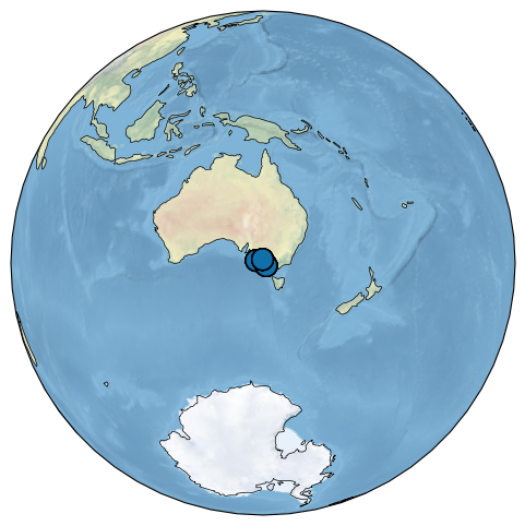

And let’s plot the timeseries!

fix,ax = mgs.stackplot(v_shift_factor = 2)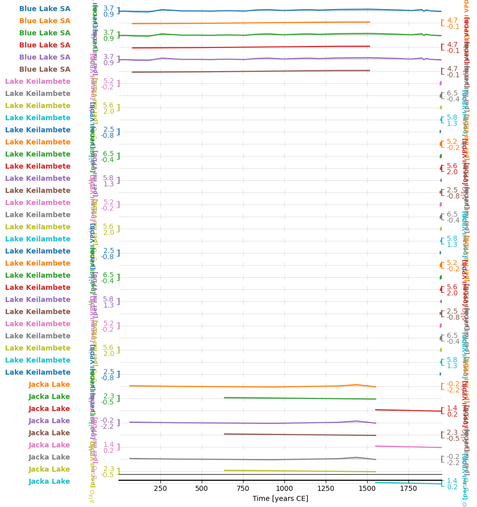

Many of these records are short!