Chapter 7 Regression and Calibration-in-time
In this chapter, we will replicate the analysis of (Boldt et al. 2015), performing age-uncertain calibration-in-time on a chlorophyll reflectance record from northern Alaska, using geoChronR.
The challenge of age-uncertain calibration-in-time is that age uncertainty affects both the calibration model (the relation between the proxy data and instrumental data) and the reconstruction (the timing of events in the reconstruction). geoChronR simplifies handling these issues.
Let’s start by loading the packages we’ll need.
library(lipdR) #to read and write LiPD files
library(geoChronR) #of course
library(readr) #to load in the instrumental data we need
library(ggplot2) #for plotting
7.1 Load the LiPD file
OK, we’ll begin by loading in the Kurupa Lake record from (Boldt et al. 2015).
K <- lipdR::readLipd("http://lipdverse.org/geoChronR-examples/Kurupa.Boldt.2015.lpd")## [1] "reading: Kurupa.Boldt.2015.lpd"7.1.1 Check out the contents
sp <- plotSummary(K,paleo.data.var = "RABD",summary.font.size = 6)## [1] "Found it! Moving on..."
## [1] "Found it! Moving on..."
## [1] "Found it! Moving on..."
## [1] "Found it! Moving on..."
## [1] "Found it! Moving on..."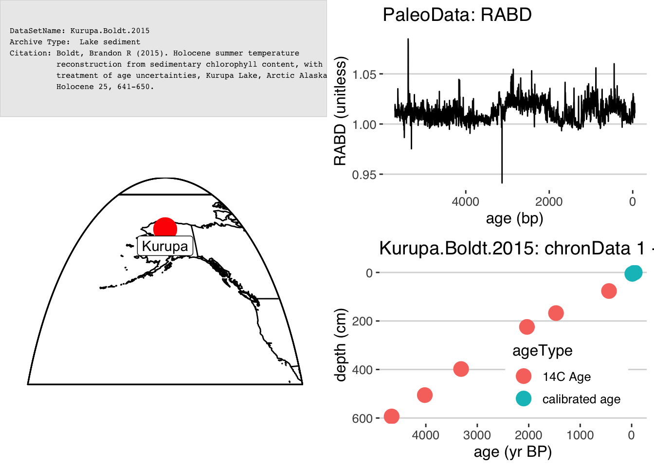
print(sp)## TableGrob (4 x 4) "arrange": 4 grobs
## z cells name grob
## 1 1 (1-1,1-2) arrange gTree[GRID.gTree.19188]
## 2 2 (1-2,3-4) arrange gtable[layout]
## 3 3 (2-4,1-2) arrange gtable[layout]
## 4 4 (3-4,3-4) arrange gtable[layout]7.2 Create an age model
K <- runBacon(K,
              lab.id.var = 'labID',
              age.14c.var = 'age14C',
              age.14c.uncertainty.var = 'age14CUncertainty',
              age.var = 'age',
              age.uncertainty.var = 'ageUncertainty',
              depth.var = 'depth',
              reservoir.age.14c.var = NULL,
              reservoir.age.14c.uncertainty.var = NULL,
              rejected.ages.var = NULL,
              bacon.acc.mean = 10,
              bacon.thick = 7,
              ask = FALSE,
              bacon.dir = "~/Cores",
              suggest = FALSE,
              close.connection = FALSE)
Exercise 7.1 In this chapter, the exercises will have conduct the analysis in a parallel universe, where you make different, but reasonable choices and see what happens.
First, create the best age model you can using either Bchron or Oxcal.
7.2.1 And plot the ensemble output
plotChron(K,age.var = "ageEnsemble",dist.scale = 0.2)## [1] "Found it! Moving on..."
## [1] "Found it! Moving on..."
## [1] "plotting your chron ensemble. This make take a few seconds..."## Scale for 'x' is already present. Adding another scale for 'x', which will replace the existing scale.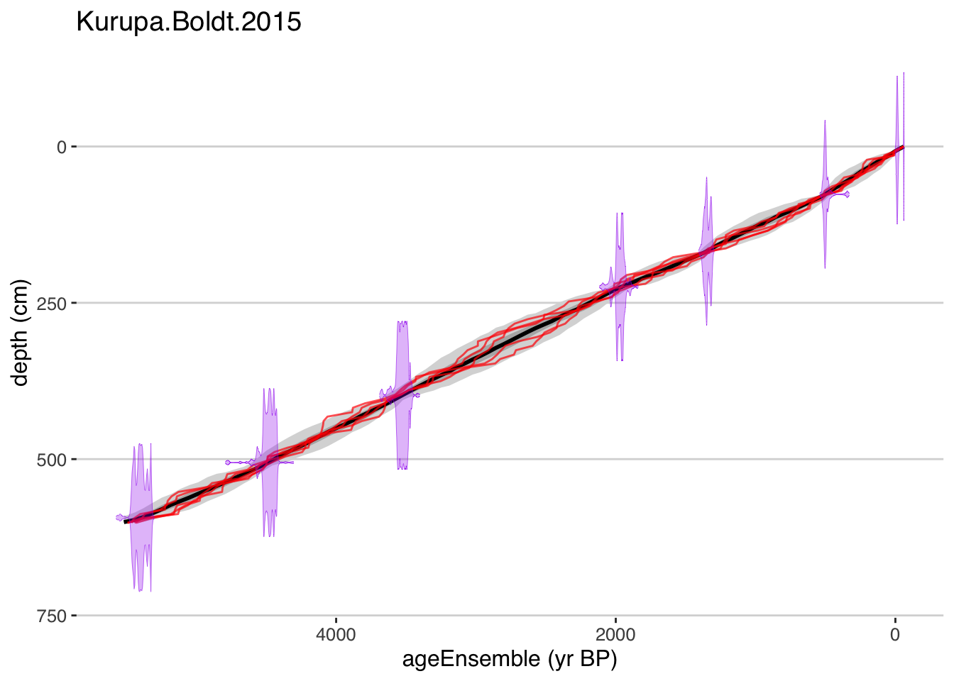
Exercise 7.2 Plot your model. How does it compare to the Bacon model?
7.3 Prepare the data
7.3.1 Map the age ensemble to the paleodata table
This is to get ensemble age estimates for each depth in the paleoData measurement table
K <- mapAgeEnsembleToPaleoData(K,age.var = "ageEnsemble")## [1] "Kurupa.Boldt.2015"
## [1] "Looking for age ensemble...."
## [1] "Found it! Moving on..."
## [1] "Found it! Moving on..."
## [1] "getting depth from the paleodata table..."
## [1] "Found it! Moving on..."7.3.2 Select the paleodata age ensemble, and RABD data that we’d like to regress and calibrate
kae <- selectData(K,"ageEnsemble")## [1] "Found it! Moving on..."rabd <- selectData(K,"RABD")## [1] "Found it! Moving on..."7.3.3 Now load in the instrumental data
kurupa.instrumental <- readr::read_csv("http://lipdverse.org/geoChronR-examples/KurupaInstrumental.csv")## Rows: 134 Columns: 2## ── Column specification ──────────────────────────────────────────────────────────────────────────────────────────────────────────
## Delimiter: ","
## dbl (2): Year (AD), JJAS Temperature (deg C)##
## ℹ Use `spec()` to retrieve the full column specification for this data.
## ℹ Specify the column types or set `show_col_types = FALSE` to quiet this message.7.3.4 Check age/time units before proceeding
kae$units## [1] "yr BP"yep, we need to convert the units from BP to AD
kae <- convertBP2AD(kae)7.3.5 Create a “variable list” for the instrumental data
kyear <- list()
kyear$values <- kurupa.instrumental[,1]
kyear$variableName <- "year"
kyear$units <- "AD"

kinst <- list()
kinst$values <- kurupa.instrumental[,2]
kinst$variableName <- "Temperature"
kinst$units <- "deg (C)"
Exercise 7.3 Repeat all of this prep work, including mapping the age uncertainties and extracting the variables.
7.3.6 Calculate an ensemble correlation between the RABD and local summer temperature data
corout <- corEns(kae,rabd,kyear,kinst,bin.step=2,percentiles = c(.05,.5,.95 ))Exercise 7.4 Calculate the correlation ensemble, but you decide to use 5-year bins instead of 2-year bins.
7.3.7 And plot the output
Note that here we use the “Effective-N” significance option as we mimic the Boldt et al. (2015) paper.
plotCorEns(corout,significance.option = "eff-n")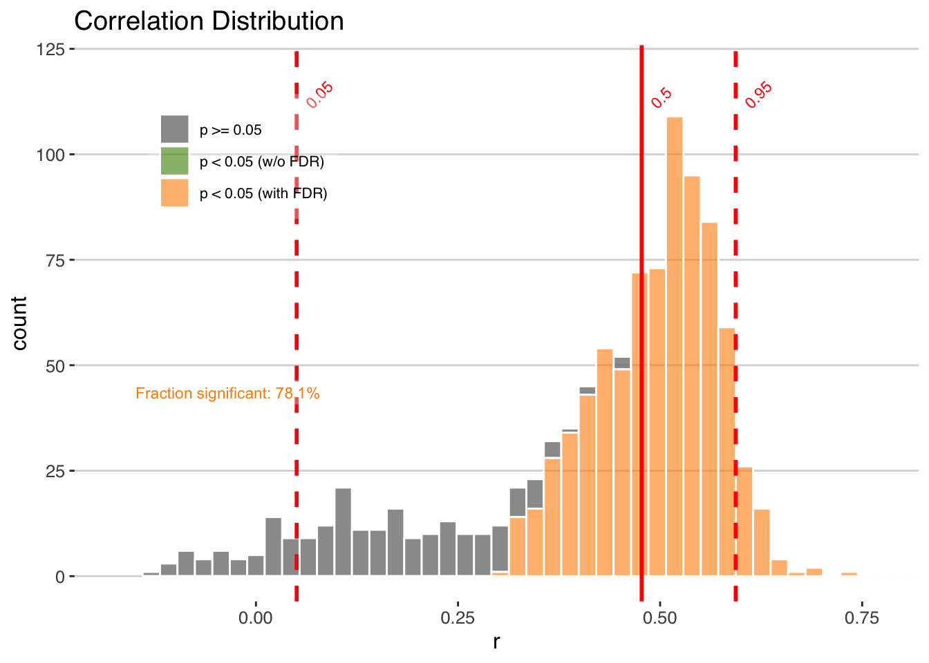
Mixed results. But encouraging enough to move forward.
Exercise 7.5 After reading Chapter ??, you know that the isospectral method is usually more reliable. Use that instead.
7.4 Perform ensemble regression
OK, you’ve convinced yourself that you want to use RABD to model temperature back through time. We can do this simply (perhaps naively) with regression, and lets do it with age uncertainty, both in the building of the model, and the reconstructing
regout <- regressEns(time.x = kae,
                    values.x = rabd,
                    time.y =kyear,
                    values.y =kinst,
                    bin.step=3,
                    gaussianize = FALSE,
                    recon.bin.vec = seq(-4010,2010,by=20))
Exercise 7.6 Again, use 5-year time steps, and also gaussianize to avoid the potential impact of skewed data
7.4.1 And plot the output
regPlots <- plotRegressEns(regout,alp = 0.01,font.size = 8)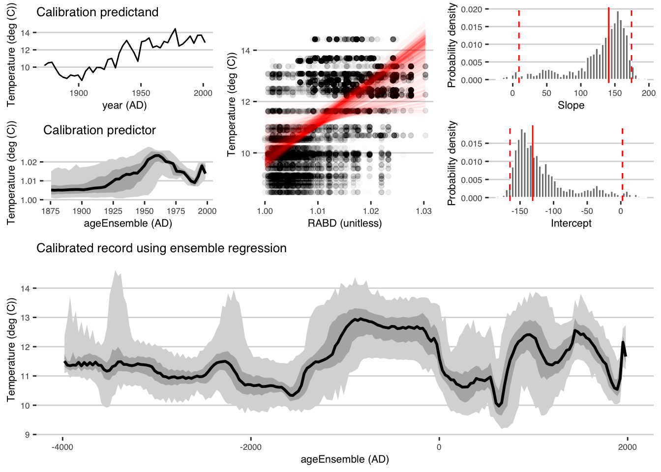
This result is consistent with that produced by Boldt et al., (2015), and was much simpler to produce with geoChronR.
7.5 Chapter project
Exercise 7.7 Plot your results. How did making different, reasonable (perhaps even better?) choices affect the final outcome of the regression?