[Fig. 5] Ensemble resampling#
Like other offline data assimilation products, the Last Millennium Reanaalysis was generated from an Ensemble Kalman Filter, which samples from a time-invariant prior distribution of climate states before judging its consistency with the observations. By definition, offline DA treats each reconstruction interval (here, years), as independent; in fact, the algorithm works identically if years are swapped, exchanged with replacement, etc. Thus, any trajectory encompassed by these distributions is technically allowed, as long as these paths preserve the distribution, particularly its low-order moments (mean, variance). However, within those loose constraints, not all resampling choices are equivalent, as some may result in a temporal structure that no longer respects what is independently known about climate variability (e.g. long-range memory). The challenge is thus to come up with resampling schemes that satisfy both constraints: - respect the posterior distribution obtained via the Kalman filter - respect independent constraints on temporal structure.
This notebooks illustrates these challenges by apply a naïve resampling strategy to the LMR ensemble, before briging other constraints to bear. It concludes with Fig 5 of the paper.
[1]:
%load_ext autoreload
%autoreload 2
import pens
import matplotlib.pyplot as plt
plt.style.use('default')
pens.set_style()
We first load the LMR v2.1 global mean surface temperature (GMST) for illustration:
[2]:
path = '../data/gmt_MCruns_ensemble_full_LMRv2.1.nc'
ens_LMR = pens.EnsembleTS().load_nc(path, var='gmt')
ens_LMR.label = 'LMR v2.1'
ens_LMR.value_name = 'GMST'
ens_LMR.value_unit = '\N{DEGREE SIGN}C'
ens_LMR.plot_qs()
[2]:
(<Figure size 1000x400 with 1 Axes>,
 <Axes: title={'center': 'LMR v2.1'}, xlabel='time', ylabel='GMST [°C]'>)
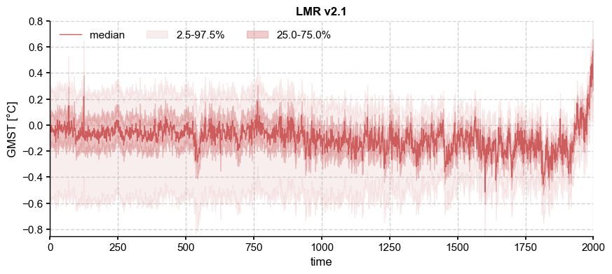
As expected from the loss of degrees of freedom due to proxy attribution, the ensemble spread increases back in time, while the ensemble median becomes increasingly flat. In other words, there is a generally inverse relationship between the temporal variance of the distribution’s central moment (the median or mean) and the variance across the ensemble at a fixed time. The individual trajectories that make up the ensemble may be visualized thus:
[3]:
ens_LMR.plot_traces(num_traces=5, alpha = 0.3, color = 'indianred')
[3]:
(<Figure size 1000x400 with 1 Axes>, <Axes: xlabel='time', ylabel='GMST [°C]'>)
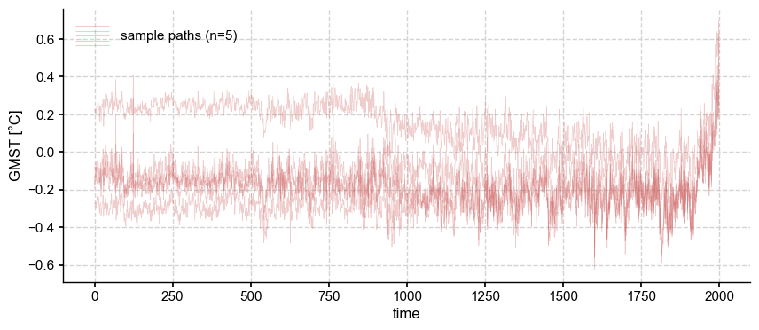
Notice that the same inverse relationship holds true for each of these ensemble members: their temporal fluctuations diminish back in time, while their get spread further apart. However, it is important to realize that these trajectories are simply labels: trajectory \(i\) is simply the \(i\)th member of this ranked ensemble, but one could just as legitimately reshuffle labels at each time step, like so:
[4]:
ens_unif = ens_LMR.random_paths(model='unif',p=5)
ens_unif.plot_traces(color='tab:green',alpha=0.3, num_traces=5)
[4]:
(<Figure size 1000x400 with 1 Axes>, <Axes: xlabel='time', ylabel='GMST [°C]'>)
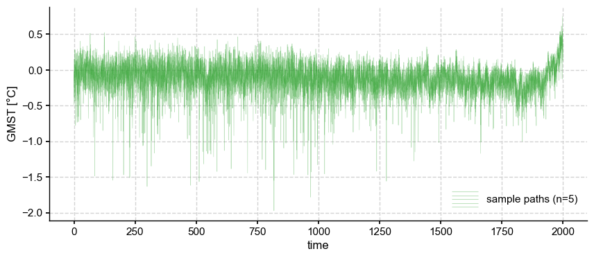
The resampling results in a much greater temporal variance, with many “cold” years from the posterior (usually, those corresponding to the aftermath of strong volcanic eruptions in the CCSM4 prior) being sampled with replacement. However, it is easy to check that the ensemble variance is unchanged:
[5]:
fig, ax = ens_LMR.get_std().plot(label='original ensemble')
ens_unif.get_std().plot(color='tab:green',ax=ax, label='uniform resampling', title='Ensemble standard deviation')
ax.legend()
[5]:
<matplotlib.legend.Legend at 0x31c049790>
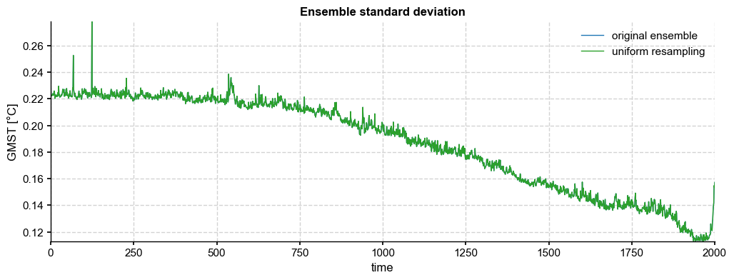
How do we satisfy these constraints while respecting the laws of physics as they apply to the temporal structure of climate variability? To do this, we need to bring in independent information.
Independent constraints on temporal structure#
This information may come in several forms, e.g. studies of instrumental climate variability, which suggest that the spectrum of GMST \(S(f)\) behaves as a power law of the form \(S(f) \propto f^{-\beta}\), where \(\beta \approx 1\) over the instrumental era (see e.g. Huybers & Curry [2005] or Zhu et al. [2019]). However, the last 150 years are too short to usefully distringhuish between several models of temporal behavior, such as long- or short-range memory (e.g. Barboza et al 2014).
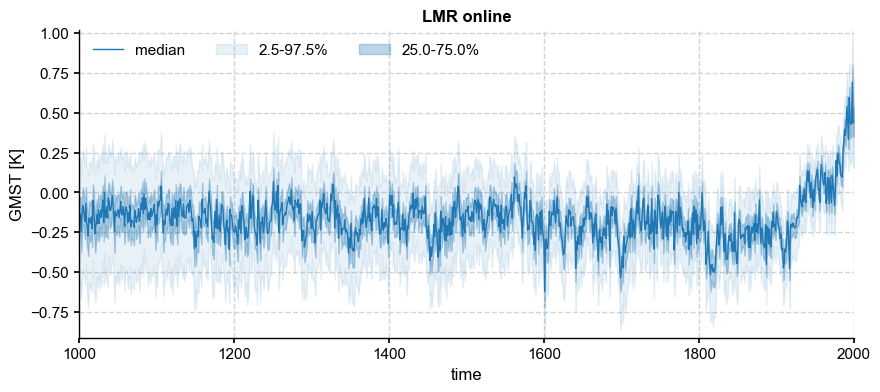
Another constraint comes from the temporal behavior of the online LMR algorithm of Perkins & Hakim [2021]. Unlike offline DA, online DA carries information from timestep to timestep via an explicit model (here, a linear inverse model, or LIM). This results in much improved reconstruction of quantities, like the ocean heat content, that are known to exhibit long-term memory but are only indirectly constrained by most climate proxy observations. To a lesser extent, Perkins & Hakim [2021] also showed improved reconstructions of GMST, with a narrower ensemble spread and more homoskedastic behavior of the ensemble mean (or median). Let us load and visualize this reconstruction:
[6]:
ens_o = pens.EnsembleTS().load_nc('../data/gmt_MCruns_ensemble_full_LMRonline.nc', var='glob_mean', time_name='year')
ens_o.label = 'LMR online'
fig, ax = ens_o.plot_qs(ylabel='GMST [K]', color = 'tab:blue')
[7]:
ens_o.plot_traces(num_traces=5, alpha=0.3, color = 'tab:blue')
[7]:
(<Figure size 1000x400 with 1 Axes>, <Axes: xlabel='time', ylabel='value'>)
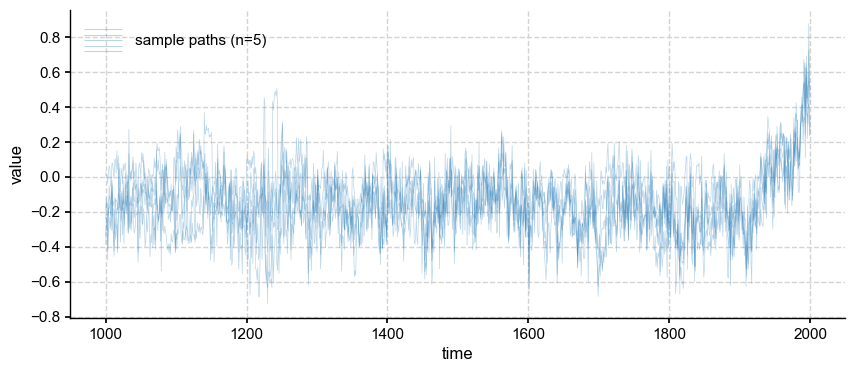
The individual traces also retain more temporal variance than their offline counterparts (see above).
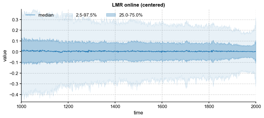
To devise a sensible resampling scheme, we analyze the spectral behavior of the online LMR to determine which timeseries model would be most appropriate. Because the ensemble mean may be viewed as a deterministic response to external forcing (e.g. explosive volcanism), we analyze the spectral behaior of residuals from the mean:
[8]:
ens_o2000 = ens_o.subsample(nsamples=ens_LMR.nEns) # downsample to the same ensemble size as LMRv2.1
ens_mean = ens_o2000.get_mean()
ens_d = ens_o2000 - ens_mean
ens_d.label = ens_o2000.label + " (centered)"
ens_d.plot_qs(color='C0')
[8]:
(<Figure size 1000x400 with 1 Axes>,
 <Axes: title={'center': 'LMR online (centered)'}, xlabel='time', ylabel='value'>)
[9]:
PSD_o = ens_d.to_pyleo(verbose=False).spectral(method='mtm',settings={'standardize':False}) # this generate a MultiplePSD object
Performing spectral analysis on individual series: 100%|██████████| 2000/2000 [00:09<00:00, 214.37it/s]
[10]:
PSD_oaa = PSD_o.anti_alias()
Applying the anti-alias filter: 100%|██████████| 2000/2000 [00:11<00:00, 175.82it/s]
[11]:
PSD_oaa.plot_envelope(curve_clr='tab:blue',shade_clr='tab:blue')
[11]:
(<Figure size 1000x400 with 1 Axes>,
 <Axes: xlabel='Period [years CE]', ylabel='PSD'>)
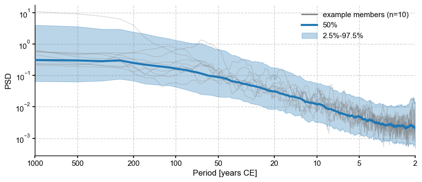
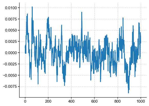
The median spectrum is not so different from an AR(1) (the aliasing at periods shorter than ~3y can be ignored). Let’s extract it, add random phase, and invert it back to the time domain.
Let’s do this as in this example
[12]:
import numpy as np
PSD_median = PSD_oaa.quantiles().psd_list[1].amplitude

nfrms = 2*ens_o.nt//2
len_ser = int((nfrms-1)/2)
interv1 = np.arange(1, len_ser+1)
interv2 = np.arange(len_ser+1, nfrms)

median_ts = np.zeros((nfrms))
ph_rnd = 2*np.pi*np.random.rand(nfrms) # random phases

magnitude = np.zeros((nfrms))
magnitude[interv1] = np.sqrt(PSD_median[interv1])
magnitude[interv2] = np.flipud(magnitude[interv1])
# Create the random phases for all the time series
FFT = magnitude*np.exp(1j*ph_rnd)
#ph_interv2 = np.conj(np.flipud(ph_interv1))

# Inverse transform
median_ts = np.real(np.fft.ifft(FFT))
plt.plot(median_ts)
[12]:
[<matplotlib.lines.Line2D at 0x31c0dfe60>]
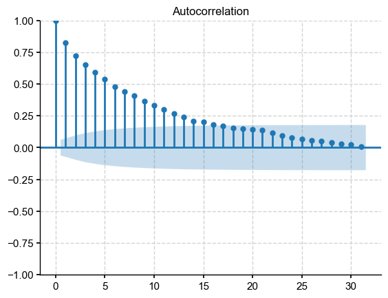
Let’s fit an autoregressive model to this series:
[13]:
import statsmodels as sm
y = median_ts
sm.graphics.tsaplots.plot_acf(y)
[13]:

[14]:
from statsmodels.tsa.ar_model import AutoReg
max_lag = 15
ar_mod = AutoReg(y, max_lag)
ar_res = ar_mod.fit(cov_type='HAC', cov_kwds={'maxlags': max_lag})  # Heteroskedasticity-autocorrelation robust covariance estimation.
print(ar_res.summary())
                            AutoReg Model Results
==============================================================================
Dep. Variable:                      y   No. Observations:                 1001
Model:                    AutoReg(15)   Log Likelihood                4914.636
Method:               Conditional MLE   S.D. of innovations              0.002
Date:                Thu, 19 Sep 2024   AIC                          -9795.273
Time:                        12:52:52   BIC                          -9712.081
Sample:                            15   HQIC                         -9763.632
                                 1001
==============================================================================
                 coef    std err          z      P>|z|      [0.025      0.975]
------------------------------------------------------------------------------
const      -1.102e-05   5.22e-05     -0.211      0.833      -0.000    9.13e-05
y.L1           0.6905      0.033     20.853      0.000       0.626       0.755
y.L2           0.0838      0.040      2.073      0.038       0.005       0.163
y.L3           0.0305      0.039      0.775      0.438      -0.047       0.108
y.L4           0.0494      0.036      1.361      0.173      -0.022       0.121
y.L5           0.0311      0.041      0.764      0.445      -0.049       0.111
y.L6          -0.0639      0.040     -1.583      0.113      -0.143       0.015
y.L7           0.0444      0.040      1.108      0.268      -0.034       0.123
y.L8           0.0137      0.041      0.336      0.737      -0.066       0.093
y.L9          -0.0149      0.041     -0.361      0.718      -0.096       0.066
y.L10          0.0082      0.039      0.210      0.834      -0.069       0.085
y.L11          0.0017      0.038      0.044      0.965      -0.072       0.076
y.L12         -0.0112      0.032     -0.347      0.729      -0.075       0.052
y.L13          0.0011      0.036      0.031      0.975      -0.069       0.071
y.L14         -0.0545      0.034     -1.593      0.111      -0.122       0.013
y.L15          0.0605      0.031      1.954      0.051      -0.000       0.121
                                    Roots
==============================================================================
                   Real          Imaginary           Modulus         Frequency
------------------------------------------------------------------------------
AR.1            -1.1744           -0.2765j            1.2065           -0.4632
AR.2            -1.1744           +0.2765j            1.2065            0.4632
AR.3            -0.9394           -0.7290j            1.1890           -0.3950
AR.4            -0.9394           +0.7290j            1.1890            0.3950
AR.5            -0.5478           -1.1161j            1.2433           -0.3226
AR.6            -0.5478           +1.1161j            1.2433            0.3226
AR.7            -0.0261           -1.1940j            1.1943           -0.2535
AR.8            -0.0261           +1.1940j            1.1943            0.2535
AR.9             0.4810           -1.1201j            1.2190           -0.1854
AR.10            0.4810           +1.1201j            1.2190            0.1854
AR.11            0.9219           -0.7930j            1.2160           -0.1131
AR.12            0.9219           +0.7930j            1.2160            0.1131
AR.13            1.0837           -0.0000j            1.0837           -0.0000
AR.14            1.1932           -0.3237j            1.2364           -0.0422
AR.15            1.1932           +0.3237j            1.2364            0.0422
------------------------------------------------------------------------------
[15]:
fig = plt.figure(figsize=(16, 9))
fig = ar_res.plot_diagnostics(fig=fig, lags=max_lag)
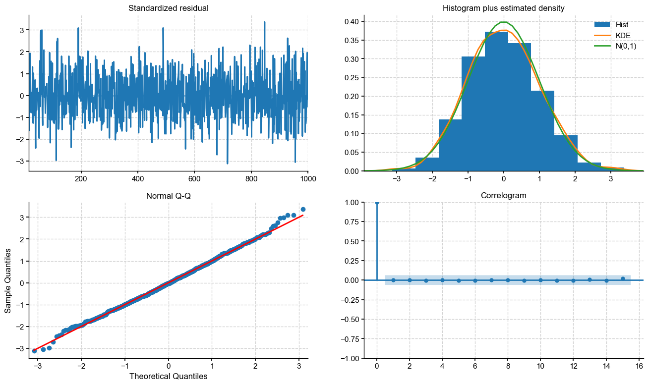
An excellent fit, except for some of the more extreme values. Let’s see what AR order is being determined automatically. From the CIs on coefficients, it looks like 2-4 would be a good choice:
[16]:
mod_sel = sm.tsa.ar_model.ar_select_order(y, maxlag=max_lag)
ar_order = len(mod_sel.ar_lags)
print("retained AR order: "+str(ar_order))
retained AR order: 2
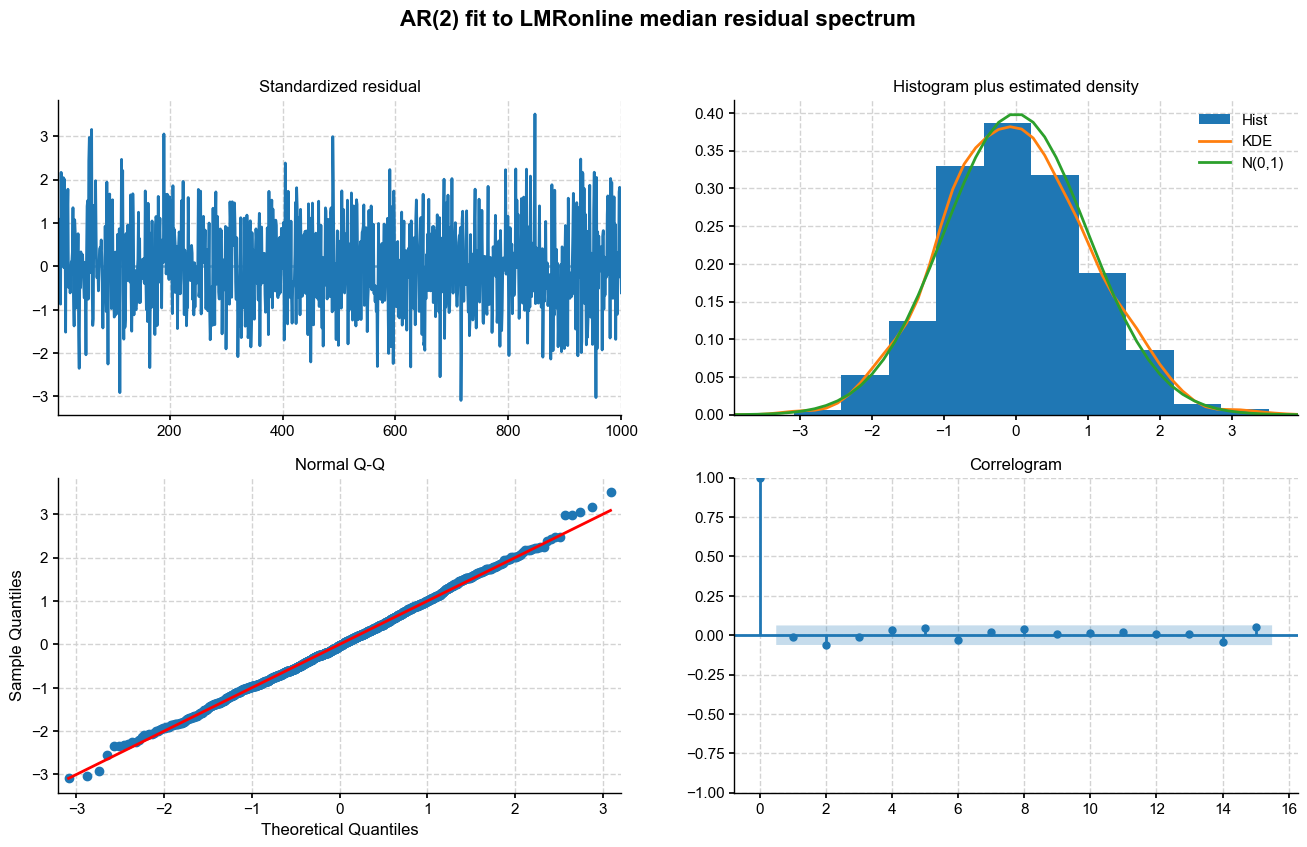
AR(2) it is. All we need to do now is pass those parameters to the ._random_paths() function in pens to simulate sensible trajectories. Before we do so, let us obtain the distribution of AR parameters from the ensemble:
[17]:
ar_mod = AutoReg(y, ar_order)
ar_res2 = ar_mod.fit(cov_kwds={'maxlags': ar_order})  # Heteroskedasticity-autocorrelation robust covariance estimation.
fig = plt.figure(figsize=(16, 9))
fig = ar_res2.plot_diagnostics(fig=fig, lags=max_lag)
fig.suptitle(f'AR({ar_order:d}) fit to LMRonline median residual spectrum',fontweight='bold',fontsize=16)
[17]:
Text(0.5, 0.98, 'AR(2) fit to LMRonline median residual spectrum')
[19]:
phi = np.empty((ens_d.nEns,ar_order+1))

for i in range(ens_d.nEns):
    ts_mod = AutoReg(ens_d.value[:,i], ar_order) # set up the model
    ts_res = ts_mod.fit(cov_type='HAC', cov_kwds={'maxlags': ar_order})  # Heteroskedasticity-autocorrelation robust covariance estimation.
    phi[i,:] = ts_res.params # export estimated parameters
Now let us plot the estimated parameters:
[20]:
import seaborn as sns
fig, axs = plt.subplots(1,2,figsize=(8,4), sharey=True)
axs = axs.flatten()
ymax = 25
for i in range(2):
    sns.kdeplot(phi[:,i+1],ax=axs[i],label='KDE over trajectories')
    axs[i].set_xlabel(r'$\hat{\phi}_'+str(i+1)+'$')

axs[1].legend(loc='upper right',fontsize=8)
fig.suptitle(f'AR({ar_order:d}) fit to detrended LMR online GMST',fontweight='bold')
[20]:
Text(0.5, 0.98, 'AR(2) fit to detrended LMR online GMST')
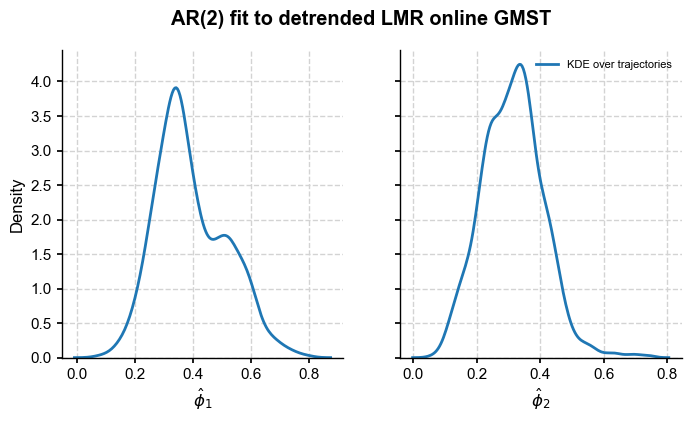
This confirms that only the first 2 AR coefficients are appreciably different from 0 in most ensemble members, so an AR(2) fit is warranted. Let us compute the mean coefficients:
[21]:
phi_o = ar_res2.params
print(phi_o)
[5.02056611e-07 7.01145589e-01 1.48088879e-01]
Resampling the offline LMR#
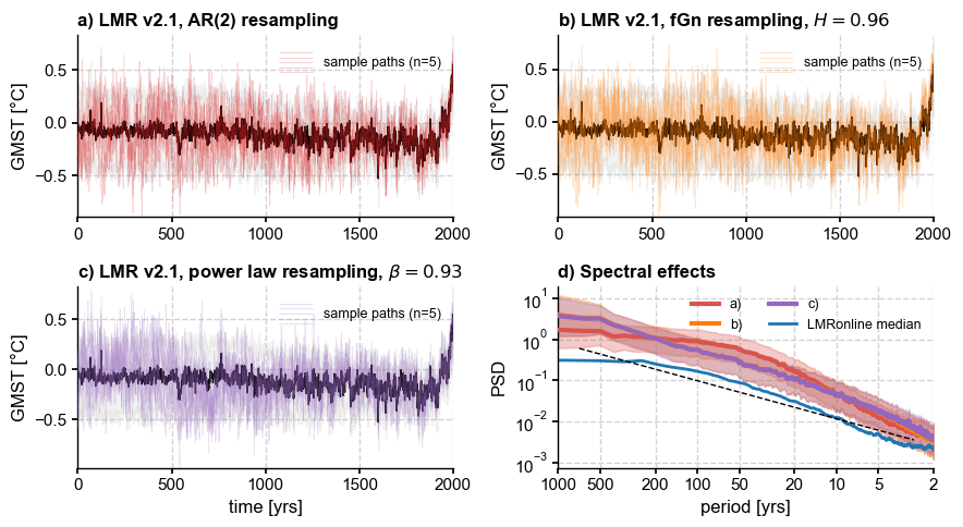
We now return to our original offline DA ensemble and try 3 timeseries models: - an autoregressive model (AR(2)) - fractional Gaussian noise (fGn) - power-law behavior
The target spectrum is the median of the distribution of detrended, standardized LMRonline spectra:
[22]:
PSD_oaa_beta  = PSD_oaa.quantiles(qs=[0.5]).beta_est()
PSD_oaa_beta.plot()
beta_o = PSD_oaa_beta.beta_est_res['beta'][0]
print(beta_o)
0.9271495631598354
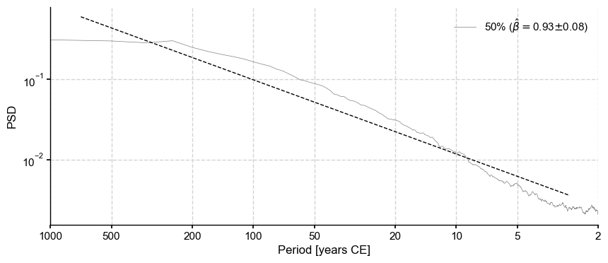
AR resampling#
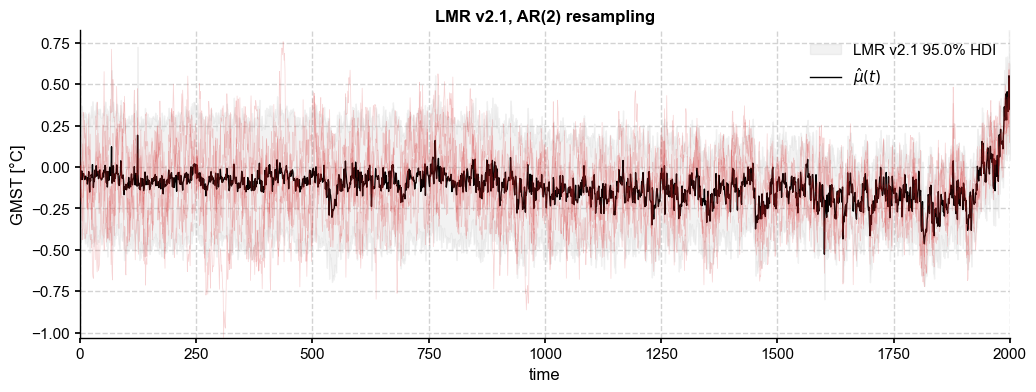
We start with an autoregressive model Because such models are stationary by construction, they cannot generate increasing variance back in time. We solve this problem (internally) by scaling the simulated AR series to unit variance, then rescaling it by the ensemble standard deviation. The result is here:
[23]:
paths_ar = ens_LMR.random_paths(model='ar',param=phi_o,p=2000)
fig, ax = ens_LMR.plot_hdi(color='silver', median=False, prob=0.95)
paths_ar.plot_traces(ax=ax,alpha=0.2,color='tab:red',num_traces=5)
ens_LMR.get_mean().plot(ax=ax, color='k', ylabel=None, label=r'$\hat{\mu}(t)$', title= ens_LMR.label + ', AR(2) resampling')
ax.legend()
100%|██████████| 2000/2000 [00:00<00:00, 10442.16it/s]
[23]:
<matplotlib.legend.Legend at 0x33b2f6a80>
[24]:
fig, ax = ens_LMR.get_std().plot(label='original ensemble')
paths_ar.get_std().plot(color='tab:red',ax=ax, label='AR(2) resampling', title='Ensemble standard deviation')
ax.legend()
[24]:
<matplotlib.legend.Legend at 0x33b010260>
[25]:
ar_ts = paths_ar.to_pyleo(verbose=False)
PSD_ar = ar_ts.spectral(method='mtm',settings={'standardize':False})
Performing spectral analysis on individual series: 100%|██████████| 2000/2000 [00:18<00:00, 110.25it/s]
[26]:
PSD_ar_aa = PSD_ar.anti_alias()
Applying the anti-alias filter: 100%|██████████| 2000/2000 [00:17<00:00, 112.48it/s]
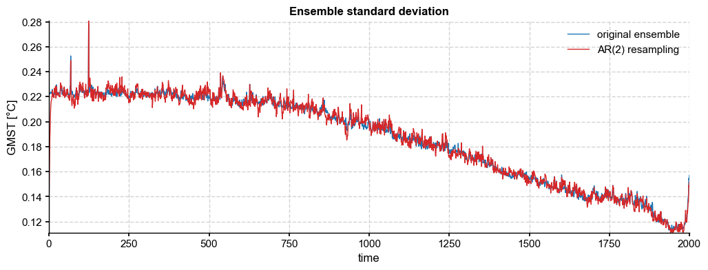
With 5000 ensemble members, we see that the AR(2) resampled ensemble achieves a sample standard deviation very close to the original, as must be the case by construction.
Power law scaling#
The last option is power-law scaling, enabled by the stochastic package. Note that under certain conditions (\(\beta = 2H-1, H<1\)), results are equivalent with fGn and the power law option.
[27]:
paths_pl = ens_LMR.random_paths(model='power-law',param=beta_o,p=2000)
fig, ax = ens_LMR.plot_hdi(color='silver', median=False, prob=0.95)
paths_pl.plot_traces(ax=ax, alpha=0.2, color='tab:purple', num_traces=10)
ens_LMR.get_mean().plot(ax=ax, color='k', ylabel=None, label=r'$\hat{\mu}(t)$',
                        title= ens_LMR.label + r', $f^{-\beta}$ resampling, ' + fr'$\beta = {beta_o:.2f}$)')
ax.legend()
100%|██████████| 2000/2000 [00:01<00:00, 1502.22it/s]
[27]:
<matplotlib.legend.Legend at 0x33591c260>
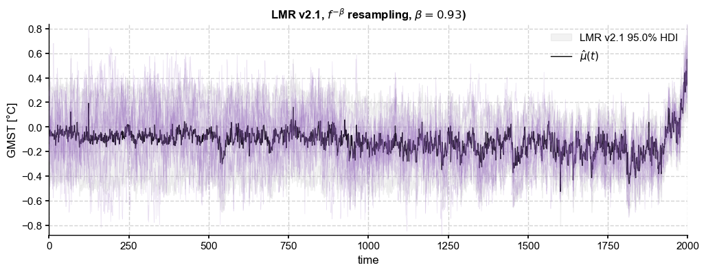
This indeed looks very similar to the fGn case. In addition, this option enables to simulate longer-memory behavior with exponents steeper than unity. For instance:
[28]:
beta = 1.2
paths_pl2 = ens_LMR.random_paths(model='power-law',param=beta,p=2000)
fig, ax = ens_LMR.plot_qs(color='silver')
paths_pl2.plot_traces(ax=ax,alpha=0.2,color='tab:purple', num_traces=10)
ens_LMR.get_mean().plot(ax=ax, color='k', ylabel=None, title= ens_LMR.label + r', $f^{-\beta}$ resampling, ' + fr'$\beta = {beta:.2f}$)')
100%|██████████| 2000/2000 [00:01<00:00, 1505.40it/s]
[28]:
<Axes: title={'center': 'LMR v2.1, $f^{-\\beta}$ resampling, $\\beta = 1.20$)'}, xlabel='time', ylabel='GMST [°C]'>
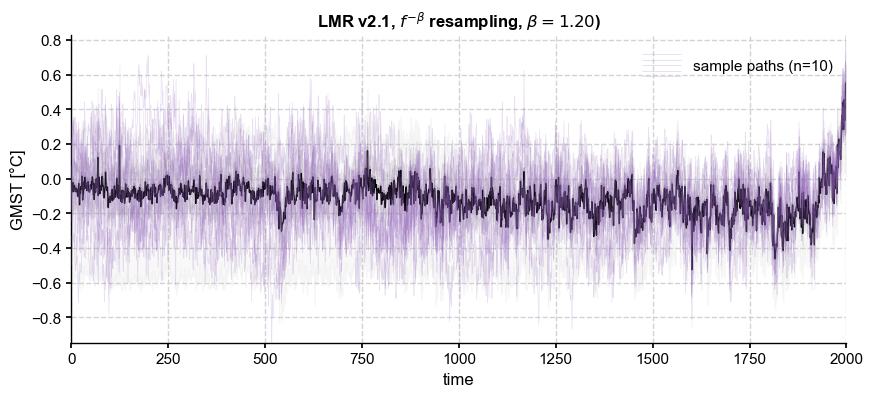
However, for \(\beta > 1\) the process is no longer stationary, which causes issues with modeling its covariance, for instance.
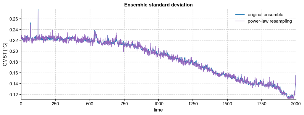
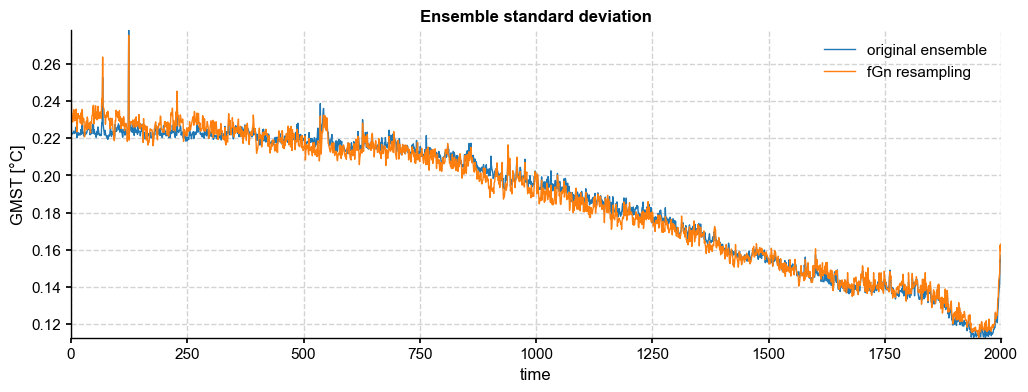
And as before, ensemble spread is preserved:
[29]:
fig, ax = ens_LMR.get_std().plot(label='original ensemble')
paths_pl.get_std().plot(color='tab:purple',ax=ax, label='power-law resampling', title='Ensemble standard deviation')
ax.legend()
[29]:
<matplotlib.legend.Legend at 0x339ffef00>
[30]:
pl_ts = paths_pl.to_pyleo(verbose=False)
PSD_pl = pl_ts.spectral(method='mtm',settings={'standardize':False})
PSD_pl_aa = PSD_pl.anti_alias()
Performing spectral analysis on individual series: 100%|██████████| 2000/2000 [00:17<00:00, 112.30it/s]
Applying the anti-alias filter: 100%|██████████| 2000/2000 [00:19<00:00, 104.27it/s]
fGn resampling#
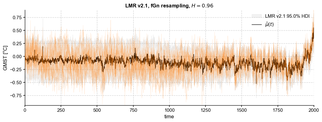
fractional Gaussian noise was popularized by Mandelbrot & Van Ness (1963) and is useful for modeling self-similar, long-memory processes. It has been abundantly used in hydrology, and is increasingly used for modeling GMST as well (see Frederiksen & Rypdal, 2017). (more background from Frederi would be helpful here)
[31]:
hurst = (beta_o+1)/2
paths_fGn = ens_LMR.random_paths(model='fGn',param=hurst,p=2000)
fig, ax = ens_LMR.plot_hdi(color='silver', median=False, prob=0.95)
paths_fGn.plot_traces(ax=ax,alpha=0.2,color='tab:orange',num_traces =10)
ens_LMR.get_mean().plot(ax=ax, color='k', ylabel=None, label=r'$\hat{\mu}(t)$',
                        title= ens_LMR.label + fr', fGn resampling, $H = {hurst:.2f}$')
ax.legend()
100%|██████████| 2000/2000 [00:00<00:00, 7529.22it/s]
[31]:
<matplotlib.legend.Legend at 0x33593d250>
[32]:
fig, ax = ens_LMR.get_std().plot(label='original ensemble')
paths_fGn.get_std().plot(color='tab:orange',ax=ax, label='fGn resampling', title='Ensemble standard deviation')
ax.legend()
[32]:
<matplotlib.legend.Legend at 0x342461f10>
[33]:
fGn_ts = paths_fGn.to_pyleo(verbose=False)
PSD_fGn = fGn_ts.spectral(method='mtm',settings={'standardize':False})
PSD_fGn_aa = PSD_fGn.anti_alias()
Performing spectral analysis on individual series: 100%|██████████| 2000/2000 [00:17<00:00, 112.20it/s]
Applying the anti-alias filter: 100%|██████████| 2000/2000 [00:17<00:00, 112.87it/s]
Finally, we summarize on a single figure:
[34]:
fig, axs = plt.subplots(2,2,figsize=(9,5))
axs = axs.flatten()
# AR resampling
ens_LMR.plot_hdi(color='silver', median=False, prob=0.95, ax= axs[0], title='')
paths_ar.plot_traces(ax=axs[0],alpha=0.2,color='tab:red',
                     lgd_kwargs={'fontsize':9}, title='')
ens_LMR.get_mean().plot(ax=axs[0], color='k', ylabel=None, label=r'$\hat{\mu}(t)$', title='')
axs[0].set_title('a) ' + ens_LMR.label + ', AR(2) resampling',
                 loc = 'left', fontweight = 'bold')
axs[0].set_xlabel('')
# fGn
ens_LMR.plot_hdi(color='silver', median=False, prob=0.95, ax= axs[1], title='')
paths_fGn.plot_traces(ax=axs[1],alpha=0.2,color='tab:orange',
                      lgd_kwargs={'fontsize':9}, title='')
ens_LMR.get_mean().plot(ax=axs[1], color='k', ylabel=None,
                        label=r'$\hat{\mu}(t)$', title='')
axs[1].set_xlabel('')
axs[1].set_title('b) ' + ens_LMR.label + fr', fGn resampling, $H = {hurst:.2f}$',
                 loc = 'left', fontweight = 'bold')
# power law
ens_LMR.plot_hdi(color='silver', median=False, prob=0.95, ax= axs[2], title='')
paths_pl.plot_traces(ax=axs[2],alpha=0.2,color='tab:purple', title='',
                     lgd_kwargs={'fontsize':9})
ens_LMR.get_mean().plot(ax=axs[2], color='k', ylabel=None, label=r'$\hat{\mu}(t)$', title='')

axs[2].set_title('c) ' + ens_LMR.label + fr', power law resampling, $\beta = {beta_o:.2f}$',
                 loc = 'left', fontweight = 'bold')
axs[2].set_xlabel('time [yrs]')
# spectra
PSD_ar_aa.plot_envelope(ax=axs[3], members_plot_num=0)
axs[3].set_title('d) Spectral effects',
                 loc = 'left', fontweight = 'bold')
PSD_fGn_aa.plot_envelope(ax=axs[3], members_plot_num=0,
                         curve_clr='tab:orange', shade_clr='tab:orange')
PSD_pl_aa.plot_envelope(ax=axs[3], members_plot_num=0,
                        curve_clr='tab:purple', shade_clr='tab:purple')
# plot median
#esm_rnd = ens_o2000.get_median()
#esm_rnd = esm_rnd.to_pyleo()
#esm_rnd_spec = esm_rnd.spectral(method ='mtm',settings={'standardize':False})
#esm_rnd_beta = esm_rnd_spec.anti_alias().beta_est() # estimate spectral exponent
#esm_rnd_beta.plot(ax=axs[3], ylabel='PSD', xlabel = 'period [yrs]')
PSD_oaa_beta.plot(ax=axs[3], ylabel='PSD', xlabel = 'period [yrs]',
                  colors = 'tab:blue', plot_kwargs={'linewidth':2})
h, l = axs[3].get_legend_handles_labels()
hdls = []; lbls =[]
hdls.append(h[0]); lbls.append('a)')
hdls.append(h[2]); lbls.append('b)')
hdls.append(h[4]); lbls.append('c)')
hdls.append(h[6]); lbls.append('LMRonline median')

axs[3].legend(handles=hdls, labels= lbls, loc='upper right', ncol=2, fontsize=9)

fig.tight_layout()
Conclusion#
pens now has 4 options for resampling the posterior ensemble of offline DA methods: 1 non-parametric method and 3 parametric ones – all distribution-preserving. As we show in the paper, naive resampling is deeply problematic, so a parametric model is necessary. However, the choice of model is subjective, and the choice of parameter requires somewhat careful thinking, so we refrain from providing one-size-fits-all defaults that would encourage users to rely on general recipes that may not
apply to the case at hand.