Getting Started with Ammonyte

Installation

Install Ammonyte using pip:

pip install ammonyte

Importing the Package

The standard convention is to import Ammonyte as amt:

import ammonyte as amt

Loading a Time Series

The central object in Ammonyte is ammonyte.Series. It extends pyleoclim.Series and serves as the starting point for all analyses.

Use the Series.from_csv() method to load a time series from a CSV file. Throughout the Ammonyte tutorials we use the NGRIP (North Greenland Ice Core Project) dataset, which contains high-resolution \(\delta^{18}O\) isotope measurements spanning the last glacial period. This dataset is well-suited for studying abrupt climate transitions such as Dansgaard-Oeschger events.

Key dataset features: - Proxy variable: \(\delta^{18}O\) isotope measurements - Units: per mil (‰) - Time scale: Thousands of years before present (kyr b2k)

ngrip = amt.Series.from_csv('../ammonyte/data/NGRIP.csv')
ngrip

Time axis values sorted in ascending order
Time axis values sorted in ascending order
{'label': 'NGRIP Ice Core Data'}

None
Age [kyr b2k]
0.05     -35.11
0.07     -34.65
0.09     -34.53
0.11     -35.29
0.13     -35.02
          ...  
122.19   -32.85
122.21   -32.66
122.23   -32.66
122.25   -32.51
122.27   -32.56
Name: δ¹⁸O [‰], Length: 6112, dtype: float64

Exploring the Series

Once loaded, you can inspect the key metadata attributes of the series:

print(f"Label:      {ngrip.label}")
print(f"Value name: {ngrip.value_name}")
print(f"Value unit: {ngrip.value_unit}")
print(f"Time name:  {ngrip.time_name}")
print(f"Time unit:  {ngrip.time_unit}")
print(f"Time range: {ngrip.time.min():.2f} – {ngrip.time.max():.2f} {ngrip.time_unit}")
print(f"Data points: {len(ngrip.time)}")

Label:      NGRIP Ice Core Data
Value name: δ¹⁸O
Value unit: ‰
Time name:  Age
Time unit:  kyr b2k
Time range: 0.05 – 122.27 kyr b2k
Data points: 6112

Visualizing the Series

Since ammonyte.Series inherits from pyleoclim.Series, you can use the .plot() method directly to visualize the time series:

fig, ax = ngrip.plot(figsize=(15, 6))
ax.set_title('NGRIP Ice Core $\delta^{18}O$ Record')
ax.grid(True, alpha=0.3)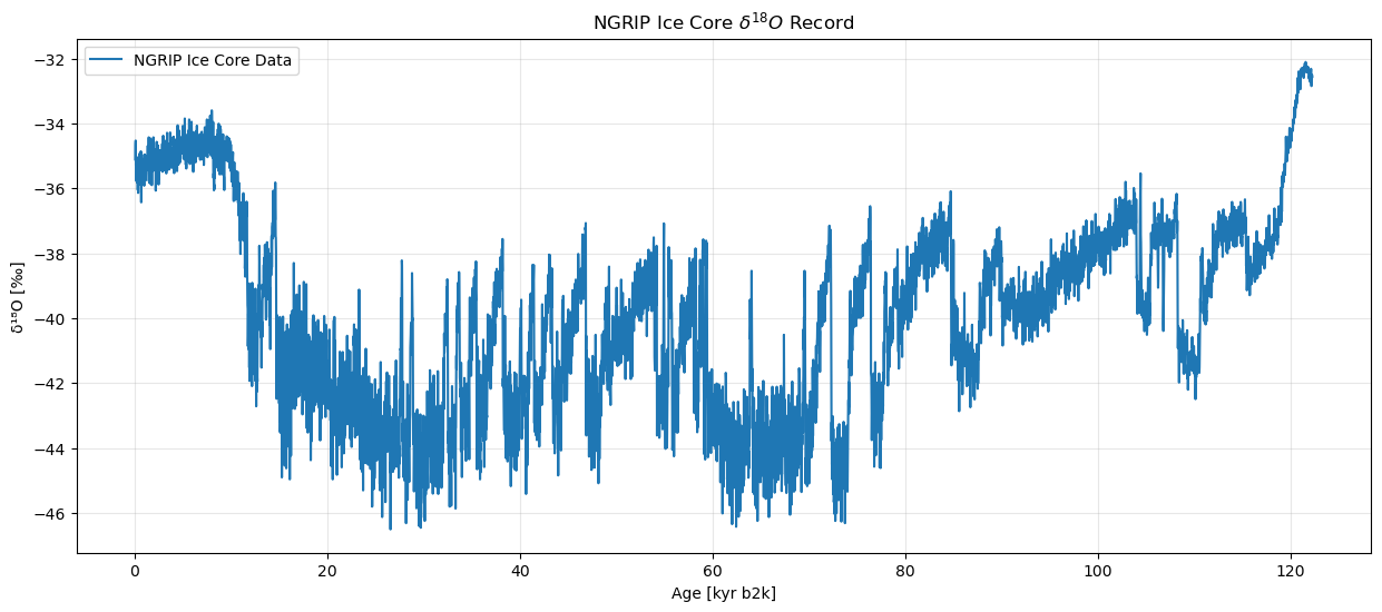

GeoSeries — Adding Geographic Context

ammonyte.GeoSeries extends Series by attaching location metadata to a geographically referenced archive. It inherits all of Ammonyte’s transition detection methods plus the geospatial methods from pyleoclim.GeoSeries, such as .map().

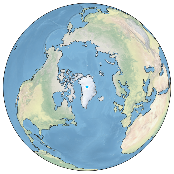
Since the NGRIP ice core was drilled at a known location in Greenland, we can wrap the series we already loaded into a GeoSeries by adding:

• lat / lon — drill site coordinates
• elevation — metres above sea level
• archiveType — type of climate archive (styles the map marker)

ngrip_geo = amt.GeoSeries(
    time=ngrip.time,
    value=ngrip.value,
    lat=75.1,
    lon=-42.32,
    elevation=3090,
    time_name=ngrip.time_name,
    time_unit=ngrip.time_unit,
    value_name=ngrip.value_name,
    value_unit=ngrip.value_unit,
    label=ngrip.label,
    archiveType='GlacierIce'
)
ngrip_geo

Time axis values sorted in ascending order
{'archiveType': 'GlacierIce', 'label': 'NGRIP Ice Core Data'}

None
Age [kyr b2k]
0.05     -35.11
0.07     -34.65
0.09     -34.53
0.11     -35.29
0.13     -35.02
          ...  
122.19   -32.85
122.21   -32.66
122.23   -32.66
122.25   -32.51
122.27   -32.56
Name: δ¹⁸O [‰], Length: 6112, dtype: float64

The .map() method places the archive on a world map, using the archiveType to style the marker:

ngrip_geo.map()

(<Figure size 1800x700 with 1 Axes>,
 {'map': <GeoAxes: xlabel='lon', ylabel='lat'>})