Detecting Tipping Points with Ammonyte’s Ruptures Wrapper

# Import libraries and packages
import ammonyte as amt
import pandas as pd
import numpy as np
import matplotlib.pyplot as plt
import time
import psutil
import os
import gc

Load the NGRIP Dataset for Tipping Point Analysis

Dataset Overview

The North Greenland Ice Core Project (NGRIP) dataset contains high-resolution paleoclimate proxy data from Greenland ice cores. This dataset is particularly valuable for studying abrupt climate transitions and tipping points in the Earth’s climate system.

Key Dataset Features: - Proxy Variable: \(\mathrm{\delta^{18}O}\) isotope measurements - Units: per mil - Time Scale: Thousands of years before present (kyr b2k)

# Load NGRIP dataset
ngrip = amt.Series.from_csv('../ammonyte/data/NGRIP.csv')

Time axis values sorted in ascending order
Time axis values sorted in ascending order

Dataset Metadata Summary

Display key metadata information from the loaded NGRIP time series to understand the dataset characteristics.

# Display metadata
print(f"Loaded NGRIP dataset: {ngrip.label}")
print(f"Time range: {ngrip.time.min():.2f} - {ngrip.time.max():.2f} {ngrip.time_unit}")
print(f"Number of data points: {len(ngrip.time)}")
print(f"Value range: {ngrip.value.min():.2f} - {ngrip.value.max():.2f} {ngrip.value_unit}")
print(f"Evenly spaced: {ngrip.is_evenly_spaced()}")

Loaded NGRIP dataset: NGRIP Ice Core Data
Time range: 0.05 - 122.27 kyr b2k
Number of data points: 6112
Value range: -46.50 - -32.11 ‰
Evenly spaced: True

NGRIP \(\mathrm{\delta^{18}O}\) Record Visualization

The plot below shows the complete NGRIP ice core record, where: - X-axis: Time in thousands of years before present (kyr b2k) - Y-axis: \(\mathrm{\delta^{18}O}\) isotope values in per mil - Interpretation: More negative values indicate colder conditions

# The NGRIP series is already loaded with proper metadata
#plot the time series to visualize the data
fig, ax = ngrip.plot(figsize=(15, 6))
ax.set_title('NGRIP Ice Core $\delta^{18}O\ [\%]$ Record')
ax.grid(True, alpha=0.3)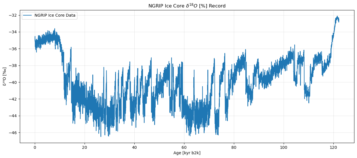

Main Rupture Analysis

This section demonstrates the complete Rupture workflow for detecting climate transitions in the NGRIP dataset. We use Pelt algorithm with l2 cost function as the recommended default configuration.

Workflow Steps: 1. Apply Rupture detection with recommended settings 2. Examine detected transitions 3. Visualize results on NGRIP time series 4. Load known Dansgaard-Oeschger (DO) events for validation 5. Quantitative validation against main DO events 6. Visualization of detected vs. known events

Step 1: Apply Rupture Detection (Default Configuration)

Recommended Configuration: - Algorithm: Pelt - Cost function: l2 - Penalty: 10

# Apply Rupture detection with recommended settings
transitions = ngrip.ruptures(algo='Pelt', cost='l2', pen=10)

Step 2: Results Summary

The output shows the number of detected change-points and details for each transition including timing, direction, and location in the time series.

# Print transition results
print(transitions)
detected_times = transitions.jump_times[~np.isnan(transitions.jump_times)]

Deterministic Transition Detection Results - NGRIP Ice Core Data | ruptures
===========================================================================
+----------+---------------------+----------------+------------------+---------------------+
| Method   |   Total Transitions |   Upward Jumps |   Downward Jumps | Series Label        |
+==========+=====================+================+==================+=====================+
| ruptures |                 108 |             41 |               67 | NGRIP Ice Core Data |
+----------+---------------------+----------------+------------------+---------------------+

Transition Details:
  1. Time: 2.77 kyr b2k, Direction: Downward, breakpoint_indices: 136.0000
  2. Time: 10.21 kyr b2k, Direction: Upward, breakpoint_indices: 508.0000
  3. Time: 10.87 kyr b2k, Direction: Upward, breakpoint_indices: 541.0000
  4. Time: 11.69 kyr b2k, Direction: Upward, breakpoint_indices: 582.0000
  5. Time: 12.77 kyr b2k, Direction: Downward, breakpoint_indices: 636.0000
  6. Time: 13.29 kyr b2k, Direction: Downward, breakpoint_indices: 662.0000
  7. Time: 14.19 kyr b2k, Direction: Downward, breakpoint_indices: 707.0000
  8. Time: 14.69 kyr b2k, Direction: Upward, breakpoint_indices: 732.0000
  9. Time: 14.99 kyr b2k, Direction: Upward, breakpoint_indices: 747.0000
  10. Time: 16.37 kyr b2k, Direction: Downward, breakpoint_indices: 816.0000
  11. Time: 17.83 kyr b2k, Direction: Upward, breakpoint_indices: 889.0000
  12. Time: 20.25 kyr b2k, Direction: Upward, breakpoint_indices: 1010.0000
  13. Time: 21.89 kyr b2k, Direction: Downward, breakpoint_indices: 1092.0000
  14. Time: 23.25 kyr b2k, Direction: Downward, breakpoint_indices: 1160.0000
  15. Time: 23.37 kyr b2k, Direction: Upward, breakpoint_indices: 1166.0000
  16. Time: 27.57 kyr b2k, Direction: Downward, breakpoint_indices: 1376.0000
  17. Time: 27.79 kyr b2k, Direction: Upward, breakpoint_indices: 1387.0000
  18. Time: 28.61 kyr b2k, Direction: Downward, breakpoint_indices: 1428.0000
  19. Time: 28.91 kyr b2k, Direction: Upward, breakpoint_indices: 1443.0000
  20. Time: 30.49 kyr b2k, Direction: Downward, breakpoint_indices: 1522.0000
  21. Time: 32.05 kyr b2k, Direction: Downward, breakpoint_indices: 1600.0000
  22. Time: 32.51 kyr b2k, Direction: Upward, breakpoint_indices: 1623.0000
  23. Time: 33.37 kyr b2k, Direction: Downward, breakpoint_indices: 1666.0000
  24. Time: 33.75 kyr b2k, Direction: Upward, breakpoint_indices: 1685.0000
  25. Time: 34.75 kyr b2k, Direction: Downward, breakpoint_indices: 1735.0000
  26. Time: 35.03 kyr b2k, Direction: Downward, breakpoint_indices: 1749.0000
  27. Time: 35.51 kyr b2k, Direction: Upward, breakpoint_indices: 1773.0000
  28. Time: 36.61 kyr b2k, Direction: Downward, breakpoint_indices: 1828.0000
  29. Time: 37.13 kyr b2k, Direction: Downward, breakpoint_indices: 1854.0000
  30. Time: 37.43 kyr b2k, Direction: Downward, breakpoint_indices: 1869.0000
  31. Time: 38.23 kyr b2k, Direction: Upward, breakpoint_indices: 1909.0000
  32. Time: 38.53 kyr b2k, Direction: Upward, breakpoint_indices: 1924.0000
  33. Time: 39.97 kyr b2k, Direction: Downward, breakpoint_indices: 1996.0000
  34. Time: 40.17 kyr b2k, Direction: Upward, breakpoint_indices: 2006.0000
  35. Time: 40.97 kyr b2k, Direction: Downward, breakpoint_indices: 2046.0000
  36. Time: 41.47 kyr b2k, Direction: Upward, breakpoint_indices: 2071.0000
  37. Time: 42.29 kyr b2k, Direction: Downward, breakpoint_indices: 2112.0000
  38. Time: 42.69 kyr b2k, Direction: Downward, breakpoint_indices: 2132.0000
  39. Time: 43.35 kyr b2k, Direction: Upward, breakpoint_indices: 2165.0000
  40. Time: 44.29 kyr b2k, Direction: Downward, breakpoint_indices: 2212.0000
  41. Time: 45.45 kyr b2k, Direction: Downward, breakpoint_indices: 2270.0000
  42. Time: 46.45 kyr b2k, Direction: Downward, breakpoint_indices: 2320.0000
  43. Time: 46.85 kyr b2k, Direction: Upward, breakpoint_indices: 2340.0000
  44. Time: 48.47 kyr b2k, Direction: Downward, breakpoint_indices: 2421.0000
  45. Time: 48.85 kyr b2k, Direction: Downward, breakpoint_indices: 2440.0000
  46. Time: 49.29 kyr b2k, Direction: Upward, breakpoint_indices: 2462.0000
  47. Time: 49.61 kyr b2k, Direction: Downward, breakpoint_indices: 2478.0000
  48. Time: 51.67 kyr b2k, Direction: Downward, breakpoint_indices: 2581.0000
  49. Time: 54.23 kyr b2k, Direction: Upward, breakpoint_indices: 2709.0000
  50. Time: 54.91 kyr b2k, Direction: Downward, breakpoint_indices: 2743.0000
  51. Time: 55.01 kyr b2k, Direction: Upward, breakpoint_indices: 2748.0000
  52. Time: 55.43 kyr b2k, Direction: Downward, breakpoint_indices: 2769.0000
  53. Time: 55.79 kyr b2k, Direction: Upward, breakpoint_indices: 2787.0000
  54. Time: 56.47 kyr b2k, Direction: Downward, breakpoint_indices: 2821.0000
  55. Time: 57.33 kyr b2k, Direction: Downward, breakpoint_indices: 2864.0000
  56. Time: 58.05 kyr b2k, Direction: Upward, breakpoint_indices: 2900.0000
  57. Time: 58.19 kyr b2k, Direction: Downward, breakpoint_indices: 2907.0000
  58. Time: 58.27 kyr b2k, Direction: Upward, breakpoint_indices: 2911.0000
  59. Time: 58.57 kyr b2k, Direction: Downward, breakpoint_indices: 2926.0000
  60. Time: 58.87 kyr b2k, Direction: Downward, breakpoint_indices: 2941.0000
  61. Time: 59.07 kyr b2k, Direction: Upward, breakpoint_indices: 2951.0000
  62. Time: 59.33 kyr b2k, Direction: Downward, breakpoint_indices: 2964.0000
  63. Time: 59.45 kyr b2k, Direction: Upward, breakpoint_indices: 2970.0000
  64. Time: 61.51 kyr b2k, Direction: Upward, breakpoint_indices: 3073.0000
  65. Time: 63.25 kyr b2k, Direction: Downward, breakpoint_indices: 3160.0000
  66. Time: 63.87 kyr b2k, Direction: Downward, breakpoint_indices: 3191.0000
  67. Time: 64.15 kyr b2k, Direction: Upward, breakpoint_indices: 3205.0000
  68. Time: 69.43 kyr b2k, Direction: Downward, breakpoint_indices: 3469.0000
  69. Time: 69.63 kyr b2k, Direction: Upward, breakpoint_indices: 3479.0000
  70. Time: 70.39 kyr b2k, Direction: Downward, breakpoint_indices: 3517.0000
  71. Time: 70.85 kyr b2k, Direction: Downward, breakpoint_indices: 3540.0000
  72. Time: 71.67 kyr b2k, Direction: Downward, breakpoint_indices: 3581.0000
  73. Time: 72.35 kyr b2k, Direction: Upward, breakpoint_indices: 3615.0000
  74. Time: 74.07 kyr b2k, Direction: Downward, breakpoint_indices: 3701.0000
  75. Time: 74.19 kyr b2k, Direction: Downward, breakpoint_indices: 3707.0000
  76. Time: 74.69 kyr b2k, Direction: Downward, breakpoint_indices: 3732.0000
  77. Time: 75.59 kyr b2k, Direction: Downward, breakpoint_indices: 3777.0000
  78. Time: 76.45 kyr b2k, Direction: Upward, breakpoint_indices: 3820.0000
  79. Time: 77.77 kyr b2k, Direction: Downward, breakpoint_indices: 3886.0000
  80. Time: 78.75 kyr b2k, Direction: Downward, breakpoint_indices: 3935.0000
  81. Time: 79.25 kyr b2k, Direction: Upward, breakpoint_indices: 3960.0000
  82. Time: 79.87 kyr b2k, Direction: Downward, breakpoint_indices: 3991.0000
  83. Time: 80.83 kyr b2k, Direction: Downward, breakpoint_indices: 4039.0000
  84. Time: 83.01 kyr b2k, Direction: Downward, breakpoint_indices: 4148.0000
  85. Time: 84.77 kyr b2k, Direction: Upward, breakpoint_indices: 4236.0000
  86. Time: 85.45 kyr b2k, Direction: Upward, breakpoint_indices: 4270.0000
  87. Time: 87.67 kyr b2k, Direction: Downward, breakpoint_indices: 4381.0000
  88. Time: 88.07 kyr b2k, Direction: Downward, breakpoint_indices: 4401.0000
  89. Time: 88.97 kyr b2k, Direction: Downward, breakpoint_indices: 4446.0000
  90. Time: 90.05 kyr b2k, Direction: Upward, breakpoint_indices: 4500.0000
  91. Time: 95.11 kyr b2k, Direction: Downward, breakpoint_indices: 4753.0000
  92. Time: 98.49 kyr b2k, Direction: Downward, breakpoint_indices: 4922.0000
  93. Time: 101.81 kyr b2k, Direction: Downward, breakpoint_indices: 5088.0000
  94. Time: 104.05 kyr b2k, Direction: Upward, breakpoint_indices: 5200.0000
  95. Time: 104.39 kyr b2k, Direction: Downward, breakpoint_indices: 5217.0000
  96. Time: 104.53 kyr b2k, Direction: Upward, breakpoint_indices: 5224.0000
  97. Time: 105.47 kyr b2k, Direction: Downward, breakpoint_indices: 5271.0000
  98. Time: 106.77 kyr b2k, Direction: Upward, breakpoint_indices: 5336.0000
  99. Time: 106.91 kyr b2k, Direction: Downward, breakpoint_indices: 5343.0000
  100. Time: 108.29 kyr b2k, Direction: Upward, breakpoint_indices: 5412.0000
  101. Time: 110.65 kyr b2k, Direction: Downward, breakpoint_indices: 5530.0000
  102. Time: 111.95 kyr b2k, Direction: Downward, breakpoint_indices: 5595.0000
  103. Time: 115.39 kyr b2k, Direction: Upward, breakpoint_indices: 5767.0000
  104. Time: 117.43 kyr b2k, Direction: Downward, breakpoint_indices: 5869.0000
  105. Time: 119.15 kyr b2k, Direction: Downward, breakpoint_indices: 5955.0000
  106. Time: 119.51 kyr b2k, Direction: Downward, breakpoint_indices: 5973.0000
  107. Time: 120.29 kyr b2k, Direction: Downward, breakpoint_indices: 6012.0000
  108. Time: 120.77 kyr b2k, Direction: Downward, breakpoint_indices: 6036.0000

Method Parameters:
  algo: Pelt
  cost: l2
  pen: 10.0
  n_bkps: None
  min_size: 2
  jump: 1
  width: None

Step 3: Transition Visualization

Display the NGRIP time series with detected change-points marked by vertical lines: - Red lines: Upward transitions (warming events) - Blue lines: Downward transitions (cooling events)

# Visualize detected transitions
fig, ax = plt.subplots(figsize=(15, 6))
transitions.plot(ax=ax, title='Rupture (PELT) Detection Results on NGRIP Ice Core Data')
plt.tight_layout()
plt.show()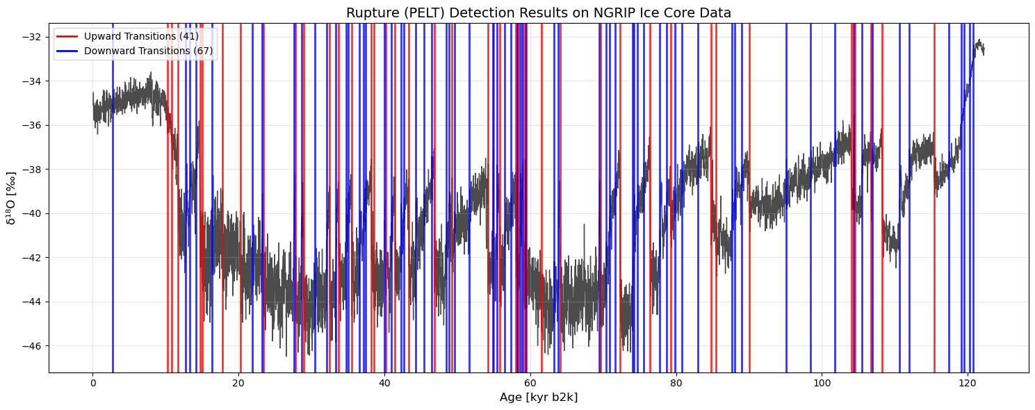

Step 4: Load Known DO Events for Validation

To validate our detection results, we compare against published Dansgaard-Oeschger (DO) events, well-documented abrupt climate transitions in the NGRIP record. These events represent rapid warming episodes followed by gradual cooling during the last glacial period.

Reference: Rasmussen et al.(2014), A stratigraphic framework for abrupt climatic changes during the Last Glacial period based on three synchronized Greenland ice-core records

Note: Event timings are subject to chronological uncertainties from annual layer counting and dating techniques, which increase with depth.

# Define D/O event chronologies as numpy arrays for analysis
do_events = pd.read_csv('../ammonyte/data/DO_events.csv', comment = '#')

main_do_events = do_events['main_kyr_b2k'].dropna().values
print(len(main_do_events)) # The length of main DO events 

all_do_events = do_events['all_kyr_b2k'].dropna().values
print(len(all_do_events))  # The length of all DO events

25
73

Step 5: Quantitative Validation Against Known DO Events

Dansgaard-Oeschger (DO) events are abrupt warming transitions, so we compare only detected upward transitions against the 25 main DO onset times from Rasmussen et al. (2014), using a ±500-year tolerance window.

# Filter to upward transitions only (DO events are abrupt warmings)
upward_mask = transitions.jump_values == 1
detected_upward = transitions.jump_times[upward_mask]
detected_upward = detected_upward[~np.isnan(detected_upward)]

# Evaluate detection performance against main DO events
results = amt.utils.evaluate_detection(detected_upward, main_do_events, tolerance=0.5)
print(results)

Detection Evaluation Metrics
============================
Metrics calculated within tolerance = 0.5

Performance Scores:
+-----------+---------+
| Metric    |   Value |
+===========+=========+
| Precision |  0.3415 |
+-----------+---------+
| Recall    |  0.56   |
+-----------+---------+
| F1 Score  |  0.4242 |
+-----------+---------+

Detection Counts:
+-----------------+---------+
| Category        |   Count |
+=================+=========+
| True Positives  |      14 |
+-----------------+---------+
| False Positives |      27 |
+-----------------+---------+
| False Negatives |      11 |
+-----------------+---------+

Summary:
  Detected: 41 | Ground Truth: 25

Step 6: Validation Visualization

This plot shows the NGRIP time series with detected upward transitions and known Dansgaard-Oeschger (DO) events overlaid. Only upward transitions are shown since DO events are defined as abrupt warming onsets.

• Red lines: Detected upward transitions
• Green dashed lines: Known DO warming events (Rasmussen et al., 2014)

fig, ax = plt.subplots(figsize=(15, 8))
ax.plot(ngrip.time, ngrip.value, color='black', linewidth=0.8, label='NGRIP $\delta^{18}\mathrm{O}$')

# Plot only upward transitions
first_up = True
for t, direction in zip(transitions.jump_times, transitions.jump_values):
    if direction > 0:
        label = 'Detected Upward Transitions' if first_up else None
        ax.axvline(x=t, color='red', alpha=0.7, linewidth=1.5, label=label)
        first_up = False

# Add DO events
for i, event_time in enumerate(main_do_events):
    if i == 0:
        ax.axvline(event_time, color='green', linestyle='--', linewidth=1.5, alpha=0.8,
                label=f'Documented DO Events by Rasmussen 2014 ({len(main_do_events)})')
    else:
        ax.axvline(event_time, color='green', linestyle='--', linewidth=1.5, alpha=0.8)

ax.set_xlabel('Time (kyr b2k)', fontsize=16)
ax.set_ylabel('$\delta^{18}\mathrm{O}$ (‰)', fontsize=16)
ax.set_title('NGRIP Upward Transitions vs. Main Dansgaard-Oeschger Events', fontsize=16)
ax.legend(loc='upper right')
ax.grid(True, alpha=0.3)
plt.tight_layout()
plt.show()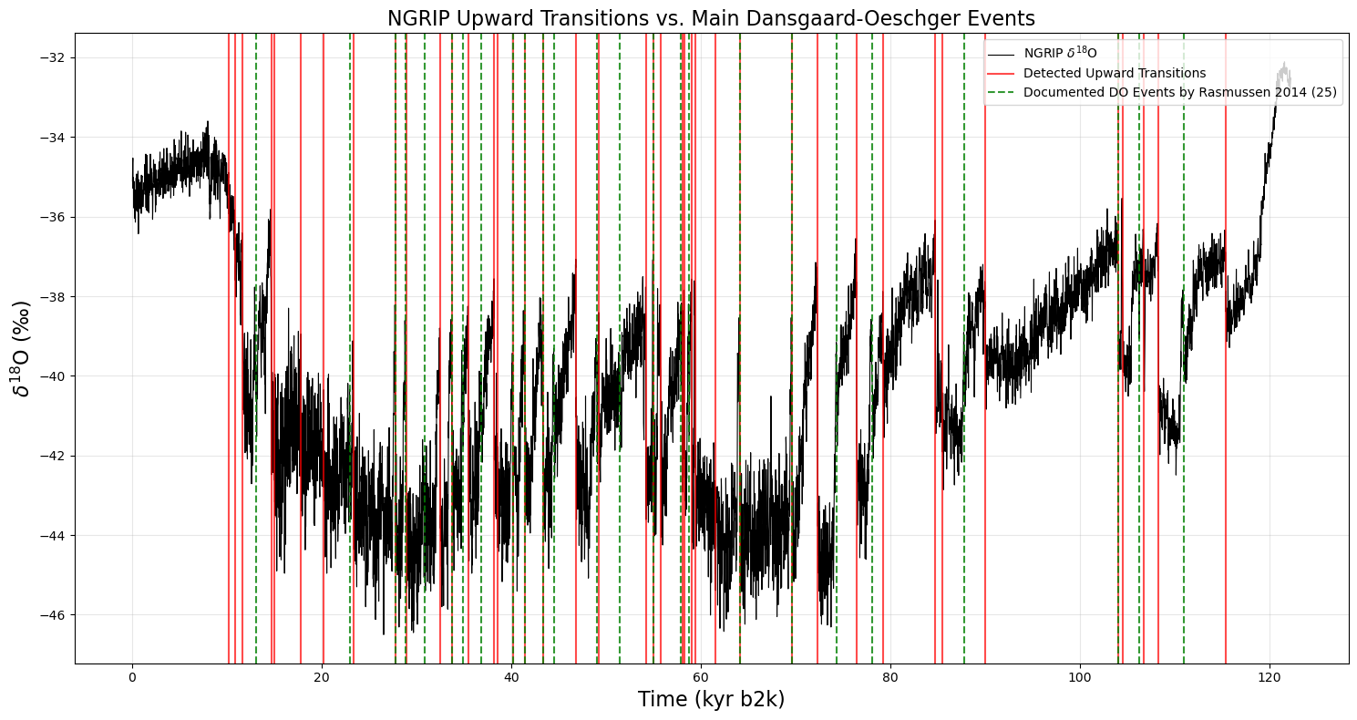

Conclusion

We see that the Pelt algorithm (l2 cost, penalty = 10) is able to identify 14 of 25 (56%) of the DO warming events documented by Rasmussen et al. (2014), with a precision of 34% (F1 = 0.42).

Pros: Highly flexible, Series.ruptures() exposes six search algorithms and multiple cost functions for different data types. Pelt automatically determines the number of change-points, so no fixed count is needed.

Major drawback: Like the KS test, ruptures algorithms detect structural breaks in statistical properties (mean, variance). They are well-suited to sharp amplitude shifts but say nothing about the dynamics. For dynamically-sensitive detection, see the LERM tutorial.

For the original ruptures library, see Truong et al. (2020).