
Working with multiple records: MultipleSeries and EnsembleSeries#
Preamble#
Introduction:#
In many cases we are interested in looking at, and thinking about, multiple time series at the same time. Here we introduce the MultipleSeries object, which serves as the basis of the various analysis techniques that apply specifically to analyzing and visualizing multiple Series objects. We also look at the EnsembleSeries, a child class of MultipleSeries with further capabilities.
Goals:#
Learn to create a
MultipleSeriesand work withcommon_time()Learn to create and customize a stackplot
Learn to create an
EnsembleSeriesLearn to visualize an
EnsembleSeries
Reading Time:
10 minutes
Keywords#
Visualization, Ensembles, stacks
Pre-requisites#
None. This tutorial assumes basic knowledge of Python. If you are not familiar with this coding language, check out this tutorial: http://linked.earth/LeapFROGS/.
Relevant Packages#
Xarray
Data Description#
LiPD files are from the Euro2k database, a subset of the PAGES 2k version 2.0.0 dataset, published by PAGES 2k Consortium, A global multiproxy database for temperature reconstructions of the Common Era. Sci Data 4, 170088 (2017). https://doi.org/10.1038/sdata.2017.88
Reconstructions of global mean surface temperature are from PAGES 2k Consortium (Neukom, R., L. A. Barboza, M. P. Erb, F. Shi, J. Emile-Geay, M. N. Evans, J. Franke, D. S. Kaufman, L. Lücke, K. Rehfeld, A. Schurer, F. Zhu, S. Br ̈onnimann, G. J. Hakim, B. J. Henley, F. C. Ljungqvist, N. McKay, V. Valler, and L. von Gunten), 2019: Consistent multidecadal variability in global temperature reconstructions and simulations over the common era, Nature Geoscience, 12(8), 643–649, https://doi.org/10.1038/s41561-019-0400-0.
Demonstration#
First, we import our favorite package:
%load_ext watermark
import pyleoclim as pyleo
import xarray as xr
%load_ext watermark
from pylipd.lipd import LiPD
The watermark extension is already loaded. To reload it, use:
  %reload_ext watermark
MultipleSeries#
Load a sample dataset#
For more details on working with LiPD files, check out the pylipd tutorials. Briefly, below we load the LiPD files located in the Euro2k directory and then create a list of those records taken from corals.
D = LiPD()

D.load_from_dir('../data/Euro2k')

timeseries,df = D.get_timeseries(D.get_all_dataset_names(),to_dataframe=True)
Loading 31 LiPD files
100%|██████████| 31/31 [00:00<00:00, 46.39it/s]
Loaded..
Extracting timeseries from dataset: Ocn-RedSea.Felis.2000 ...
Extracting timeseries from dataset: Arc-Forfjorddalen.McCarroll.2013 ...
Extracting timeseries from dataset: Eur-Tallinn.Tarand.2001 ...
Extracting timeseries from dataset: Eur-CentralEurope.Dobrovoln_.2009 ...
Extracting timeseries from dataset: Eur-EuropeanAlps.B_ntgen.2011 ...
Extracting timeseries from dataset: Eur-CentralandEasternPyrenees.Pla.2004 ...
Extracting timeseries from dataset: Arc-Tjeggelvas.Bjorklund.2012 ...
Extracting timeseries from dataset: Arc-Indigirka.Hughes.1999 ...
Extracting timeseries from dataset: Eur-SpannagelCave.Mangini.2005 ...
Extracting timeseries from dataset: Ocn-AqabaJordanAQ19.Heiss.1999 ...
Extracting timeseries from dataset: Arc-Jamtland.Wilson.2016 ...
Extracting timeseries from dataset: Eur-RAPiD-17-5P.Moffa-Sanchez.2014 ...
Extracting timeseries from dataset: Eur-LakeSilvaplana.Trachsel.2010 ...
Extracting timeseries from dataset: Eur-NorthernSpain.Mart_n-Chivelet.2011 ...
Extracting timeseries from dataset: Eur-MaritimeFrenchAlps.B_ntgen.2012 ...
Extracting timeseries from dataset: Ocn-AqabaJordanAQ18.Heiss.1999 ...
Extracting timeseries from dataset: Arc-Tornetrask.Melvin.2012 ...
Extracting timeseries from dataset: Eur-EasternCarpathianMountains.Popa.2008 ...
Extracting timeseries from dataset: Arc-PolarUrals.Wilson.2015 ...
Extracting timeseries from dataset: Eur-LakeSilvaplana.Larocque-Tobler.2010 ...
Extracting timeseries from dataset: Eur-CoastofPortugal.Abrantes.2011 ...
Extracting timeseries from dataset: Eur-TatraMountains.B_ntgen.2013 ...
Extracting timeseries from dataset: Eur-SpanishPyrenees.Dorado-Linan.2012 ...
Extracting timeseries from dataset: Eur-FinnishLakelands.Helama.2014 ...
Extracting timeseries from dataset: Eur-Seebergsee.Larocque-Tobler.2012 ...
Extracting timeseries from dataset: Eur-NorthernScandinavia.Esper.2012 ...
Extracting timeseries from dataset: Arc-GulfofAlaska.Wilson.2014 ...
Extracting timeseries from dataset: Arc-Kittelfjall.Bjorklund.2012 ...
Extracting timeseries from dataset: Eur-L_tschental.B_ntgen.2006 ...
Extracting timeseries from dataset: Eur-Stockholm.Leijonhufvud.2009 ...
Extracting timeseries from dataset: Arc-AkademiiNaukIceCap.Opel.2013 ...
indices = {key:[] for key in timeseries.keys()}

for key,ts_list in timeseries.items():
    for idx,ts_dict in enumerate(ts_list):
        if 'archiveType' in ts_dict.keys(): #check that it is available to avoid errors on the loop
            if ts_dict['archiveType'] == 'Coral': #if it's a coral, then proceed to the next step
                if ts_dict['paleoData_variableName'] in ['d13C','d18O']:
                    indices[key].append(idx)

ts_list_euro_coral =[]

for key,index_list in indices.items():

    if not index_list:
        continue
    else:
        pass

    for idx in index_list:
        ts_dict = timeseries[key][idx]
        series_tmp = pyleo.Series(
                                time=ts_dict['year'],
                                value=ts_dict['paleoData_values'],
                                time_name='Years',
                                time_unit=ts_dict['yearUnits'],
                                value_name=ts_dict['paleoData_variableName'],
                                value_unit=ts_dict['paleoData_units'],
                                label=key
                                )
        ts_list_euro_coral.append(series_tmp)
Time axis values sorted in ascending order
Time axis values sorted in ascending order
Time axis values sorted in ascending order
Time axis values sorted in ascending order
Time axis values sorted in ascending order
To create a pyleo.MultipleSeries, simply pass a collection of pyleo.Series objects. (In this case, we are passing a
list
of
pyleo.LipdSeries, which works because a pyleo.LipdSeries is a special type of pyleo.Series.)
redsea_corals = pyleo.MultipleSeries(ts_list_euro_coral, label='Red Sea Corals', time_unit='year CE')
There are a number of useful methods available to quickly learn about our set of records.
For example, .equal_length() is a quick way to see if the records are the same length.
redsea_corals.equal_lengths()
(False, [1468, 107, 107, 206, 206])
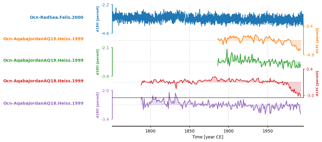
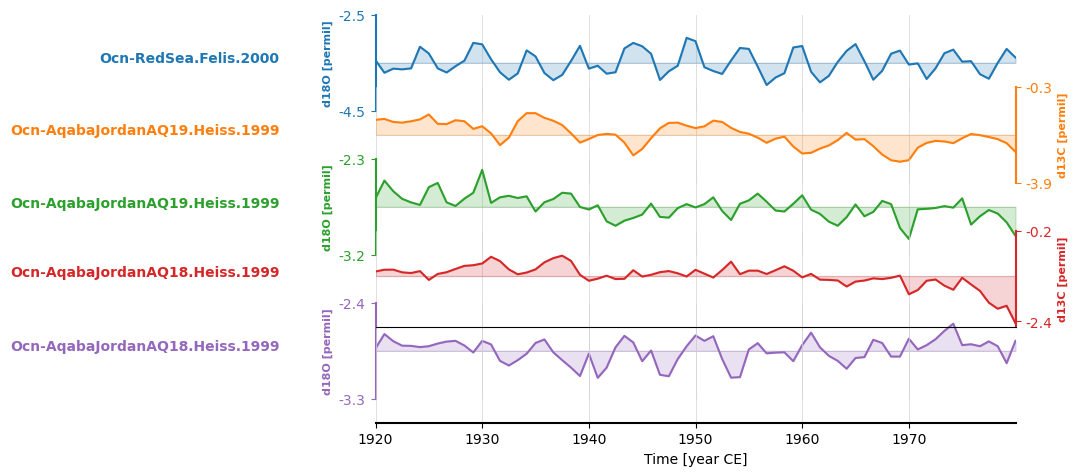
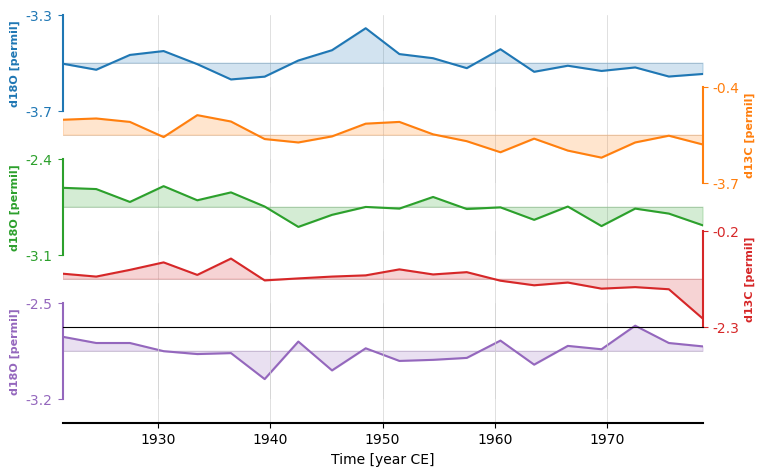
.equal_lengths() usefully returns a True/False and the length of each record. In this case, they are not, which we can visualize by plotting them using .stackplot():
fig, ax = redsea_corals.stackplot()
Pyleoclim also allows you to plot the MultipleSeries as warming stripes:
fig,ax = redsea_corals.stripes(ref_period=(1950,2000), figsize=(8,4))
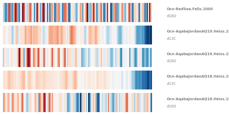
Remember that \(\delta^{18}O\) becomes more negative as temperature increases, hence the warming stripes on this figure are “reversed”, with warmer temperatures in blue. You could also use the .flip() function to flip the y axis of individual Series objects. Finally, note that stripes() admits several colormaps. For instance:
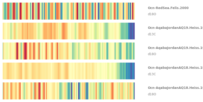
fig,ax = redsea_corals.stripes(ref_period=(1950,2000), figsize=(8,4), cmap='Spectral_r')
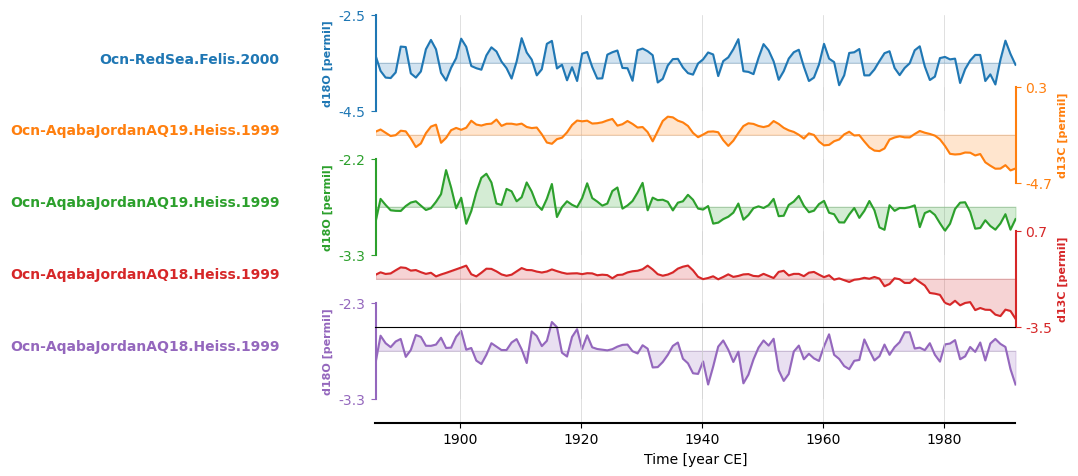
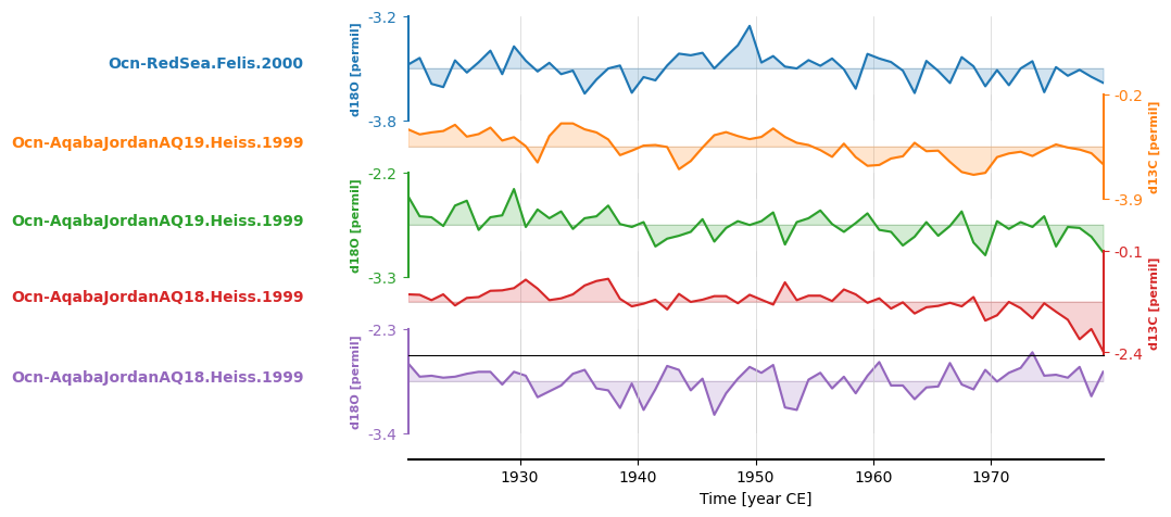
If we wanted to place the records on a shared time axis with a common sampling frequency and focus on the interval shared by all
records in the MultipleSeries, we could apply .common_time().
redsea_corals_ct = redsea_corals.common_time()
fig, ax = redsea_corals_ct.stackplot()
By default, .common_time() interpolates and infers spacing from the records involved and returns a MultipleSeries that spans the full shared interval. However, these parameters can be tuned. For example, in addition to interpolation, it also allows binning and a Gaussian kernel. Downsampling is a simple matter of specifying the preferred value for step, and focusing in on a subinterval of the shared interval is only a matter of assigning relevant date values to start and stop.
For more information see
documentation on common_time().
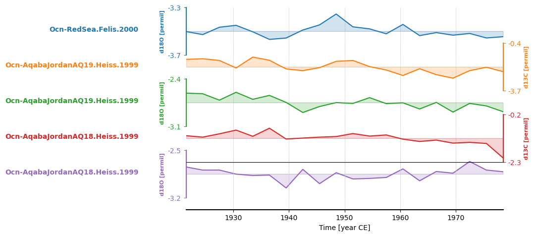
redsea_corals_ct = redsea_corals.common_time(start=1920, stop=1980)
fig, ax = redsea_corals_ct.stackplot()
redsea_corals_ct = redsea_corals.common_time(method = 'bin', step=1, start=1920, stop=1980)
fig, ax = redsea_corals_ct.stackplot()
redsea_corals_ct = redsea_corals.common_time(step=3, start=1920, stop=1980, method='gkernel')
fig, ax = redsea_corals_ct.stackplot()
Tuning a stackplot#
Labels#
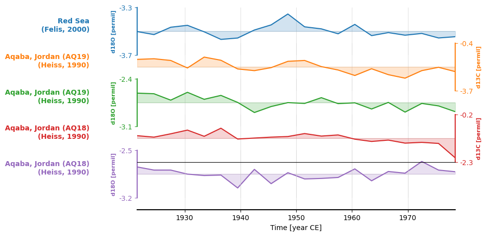
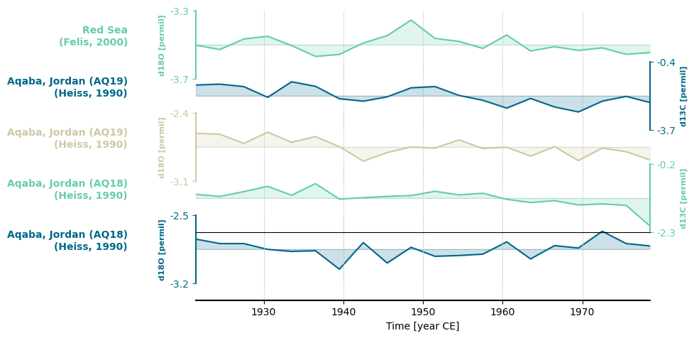
The labels attached to each record in the stackplot above are a bit unweildy. To make them a bit more readable, we
can pass a list of labels to labels.
fig, ax = redsea_corals_ct.stackplot(labels=['Red Sea\n(Felis, 2000)',
                                             'Aqaba, Jordan (AQ19)\n(Heiss, 1990)',
                                             'Aqaba, Jordan (AQ19)\n(Heiss, 1990)',
                                             'Aqaba, Jordan (AQ18)\n(Heiss, 1990)',
                                             'Aqaba, Jordan (AQ18)\n(Heiss, 1990)'])
Alternatively, we could remove the labels entirely by setting labels to None.
fig, ax = redsea_corals_ct.stackplot(labels=None)
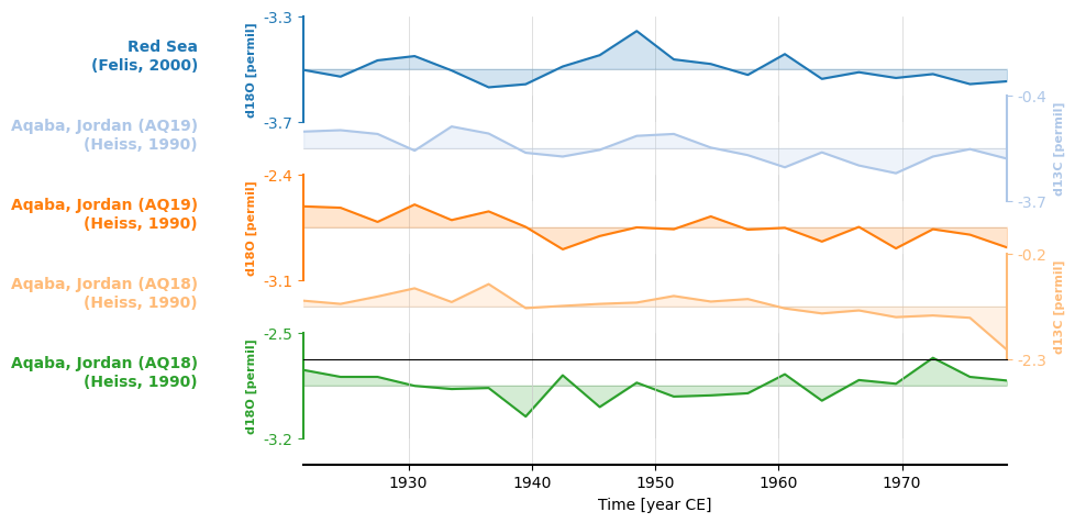
Color#
If we want to change the colors to a set other than the default
(tab10), we can pass a list of Python
supported color codes (one or more strings of hex code, or tuples of rgba values)) to colors. If the list is
shorter than the number of records, the plot will simply cycle through them.
fig, ax = redsea_corals_ct.stackplot(labels=['Red Sea\n(Felis, 2000)',
                                             'Aqaba, Jordan (AQ19)\n(Heiss, 1990)',
                                             'Aqaba, Jordan (AQ19)\n(Heiss, 1990)',
                                             'Aqaba, Jordan (AQ18)\n(Heiss, 1990)',
                                             'Aqaba, Jordan (AQ18)\n(Heiss, 1990)'],
                                                colors=['#66CDAA', '#00688B', '#CDC9A5'])
Alternatively, we can pass a color map and let pyleoclim figure out how to specify the colors. More information about
color maps is available in this Matplotlib tutorial
on the subject. While it is possible to create colormaps from scratch, let’s go with tab20. (Custom colormaps
are left as an exercise to the intrepid reader.)
fig, ax = redsea_corals_ct.stackplot(labels=['Red Sea\n(Felis, 2000)',
                                             'Aqaba, Jordan (AQ19)\n(Heiss, 1990)',
                                             'Aqaba, Jordan (AQ19)\n(Heiss, 1990)',
                                             'Aqaba, Jordan (AQ18)\n(Heiss, 1990)',
                                             'Aqaba, Jordan (AQ18)\n(Heiss, 1990)'],
                                              cmap='tab20')
Using shorthands#
Notice how earlier we used the pyleo.MultipleSeries([list]) syntax to bundle a list of Series objects into a MultipleSeries object.
Here we showcase easier shorthands to create and manipulate MultipleSeries objects. First, let’s load a few records covering part of the Plio-Pleistocene:
co2ts = pyleo.utils.load_dataset('AACO2')
lr04 = pyleo.utils.load_dataset('LR04')
edc = pyleo.utils.load_dataset('EDC-dD')
We then create a MultipleSeries object using the & shorthand:
ms = lr04.flip() & edc & co2ts
type(ms)
The two series have different lengths, left: 2115 vs right: 1901
Metadata are different:
value_unit property -- left: ‰, right: ppm
value_name property -- left: $\delta^{18} \mathrm{O}$ x (-1), right: $CO_2$
label property -- left: LR04 benthic stack, right: EPICA Dome C CO2
archiveType property -- left: MarineSediment, right: GlacierIce
importedFrom property -- left: None, right: https://www.ncei.noaa.gov/pub/data/paleo/icecore/antarctica/antarctica2015co2composite.txt
The two series have different lengths, left: 5785 vs right: 1901
Metadata are different:
lat property -- left: -75.1011, right: None
lon property -- left: 123.3478, right: None
elevation property -- left: 3233, right: None
time_unit property -- left: y BP, right: ky BP
value_unit property -- left: ‰, right: ppm
value_name property -- left: $\delta \mathrm{D}$, right: $CO_2$
label property -- left: EPICA Dome C dD, right: EPICA Dome C CO2
sensorType property -- left: ice sheet, right: None
observationType property -- left: hydrogen isotopes, right: None
importedFrom property -- left: https://www.ncei.noaa.gov/pub/data/paleo/icecore/antarctica/epica_domec/edc3deuttemp2007.txt, right: https://www.ncei.noaa.gov/pub/data/paleo/icecore/antarctica/antarctica2015co2composite.txt
control_archiveType property -- left: False, right: None
pyleoclim.core.multipleseries.MultipleSeries
Do not be alarmed by this text output ; it merely checks that the series are different prior to putting them together, so as to avoid duplicates. As with Series, there are two display options. The first is a barebones visualization of the associated dataframe:
ms
                         LR04 benthic stack  EPICA Dome C dD  EPICA Dome C CO2
datetime
-5318046-05-22 11:46:11               -2.91              NaN               NaN
-5313046-05-20 11:37:24               -2.84              NaN               NaN
-5308046-05-19 11:28:37               -2.79              NaN               NaN
-5303046-05-17 11:19:50               -2.79              NaN               NaN
-5298046-05-16 11:11:03               -2.91              NaN               NaN
...                                     ...              ...               ...
1993-01-29 15:12:50                     NaN              NaN            353.95
1994-05-30 09:44:42                     NaN              NaN            357.11
1996-04-12 09:48:54                     NaN              NaN            359.65
1997-12-31 15:00:46                     NaN              NaN            361.78
2001-01-11 07:25:32                     NaN              NaN            368.02

[9801 rows x 3 columns]
The second will look like a nicely formatted table in the Jupyter context:
ms.view()
| LR04 benthic stack | EPICA Dome C dD | EPICA Dome C CO2 | |
|---|---|---|---|
| Age | |||
| -0.05103 | NaN | NaN | 368.02 |
| -0.04800 | NaN | NaN | 361.78 |
| -0.04628 | NaN | NaN | 359.65 |
| -0.04441 | NaN | NaN | 357.11 |
| -0.04308 | NaN | NaN | 353.95 |
| ... | ... | ... | ... |
| 797408.00000 | NaN | -440.20 | NaN |
| 798443.00000 | NaN | -439.00 | NaN |
| 799501.00000 | NaN | -441.10 | NaN |
| 800589.00000 | NaN | -441.42 | NaN |
| 801662.00000 | NaN | -440.90 | NaN |
9801 rows × 3 columns
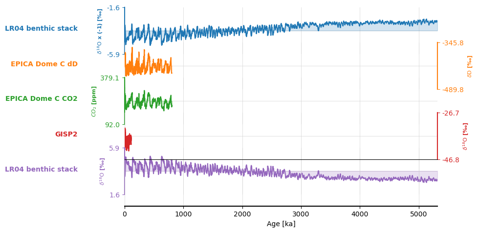
Notice how this option formats the index as a more recognizable variable (in this case, the age, in years BP here). However, when plotted, the units of the first series are used:
ms.standardize().plot()
(<Figure size 1000x400 with 1 Axes>, <Axes: xlabel='Age [ka]', ylabel='value'>)
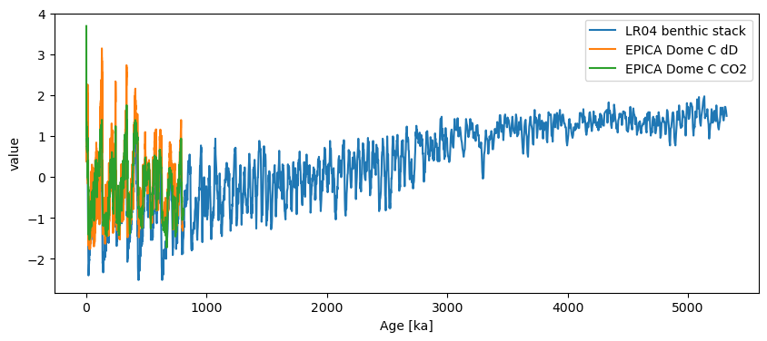
This correctly shows up as “ka” in this case. If some of the series in the collection have different units, all that needs to be done is to apply convert_time_unit() prior to plotting. Notice that we had flipped the LR04 values upon creating the object, so the values of all series in the MultipleSeries vary in unison.
Adding a series to a MultipleSeries object:#
You could add another series to the previous collection using pyleo.MultipleSeries(), but it would be rather tedious.
As of version 0.11.0, this operation can now be done with the “+” operator, which is understood to mean: “add this Series to the existing MultipleSeries object”. The method will confirm that you are not adding a series that is already in the MultipleSeries object by comparing it to the contents of the object, pairwise. For instance, let’s add the GISP2 timeseries:
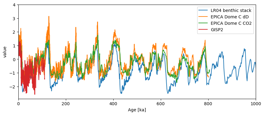
gisp2 = pyleo.utils.load_dataset('GISP2')
ms3 = ms + gisp2
fig, ax = ms3.standardize().plot()
ax.set_xlim([0, 1000]) # plot only over the past 1 Ma
The two series have different lengths, left: 2115 vs right: 1390
Metadata are different:
time_unit property -- left: ky BP, right: yr BP
value_name property -- left: $\delta^{18} \mathrm{O}$ x (-1), right: $\delta^{18} \mathrm{O}$
label property -- left: LR04 benthic stack, right: GISP2
archiveType property -- left: MarineSediment, right: GlacierIce
importedFrom property -- left: None, right: https://www.ncei.noaa.gov/access/paleo-search/study/17796
The two series have different lengths, left: 5785 vs right: 1390
Metadata are different:
lat property -- left: -75.1011, right: None
lon property -- left: 123.3478, right: None
elevation property -- left: 3233, right: None
time_unit property -- left: y BP, right: yr BP
value_name property -- left: $\delta \mathrm{D}$, right: $\delta^{18} \mathrm{O}$
label property -- left: EPICA Dome C dD, right: GISP2
sensorType property -- left: ice sheet, right: None
observationType property -- left: hydrogen isotopes, right: None
importedFrom property -- left: https://www.ncei.noaa.gov/pub/data/paleo/icecore/antarctica/epica_domec/edc3deuttemp2007.txt, right: https://www.ncei.noaa.gov/access/paleo-search/study/17796
control_archiveType property -- left: False, right: None
The two series have different lengths, left: 1901 vs right: 1390
Metadata are different:
time_unit property -- left: ky BP, right: yr BP
value_unit property -- left: ppm, right: ‰
value_name property -- left: $CO_2$, right: $\delta^{18} \mathrm{O}$
label property -- left: EPICA Dome C CO2, right: GISP2
importedFrom property -- left: https://www.ncei.noaa.gov/pub/data/paleo/icecore/antarctica/antarctica2015co2composite.txt, right: https://www.ncei.noaa.gov/access/paleo-search/study/17796
(0.0, 1000.0)
Adding two MultipleSeries objects together:#
Suppose now I want to add two MultipleSeries objects together. There a shorthand for that, intuitively called “+”. Note that the “&” operator would be inappropriate here, as it means please blundle these Series objects into a MultipleSeries object. We’ll create a new MultipleSeries object called ms2, made of the original (unflipped) LR04 and GISP2:
ms2 = gisp2 & lr04
Let’s now add this to ms:
mst = ms + ms2
The two series have different lengths, left: 2115 vs right: 1390
Metadata are different:
time_unit property -- left: ky BP, right: yr BP
value_name property -- left: $\delta^{18} \mathrm{O}$ x (-1), right: $\delta^{18} \mathrm{O}$
label property -- left: LR04 benthic stack, right: GISP2
archiveType property -- left: MarineSediment, right: GlacierIce
importedFrom property -- left: None, right: https://www.ncei.noaa.gov/access/paleo-search/study/17796
The two series have different lengths, left: 5785 vs right: 1390
Metadata are different:
lat property -- left: -75.1011, right: None
lon property -- left: 123.3478, right: None
elevation property -- left: 3233, right: None
time_unit property -- left: y BP, right: yr BP
value_name property -- left: $\delta \mathrm{D}$, right: $\delta^{18} \mathrm{O}$
label property -- left: EPICA Dome C dD, right: GISP2
sensorType property -- left: ice sheet, right: None
observationType property -- left: hydrogen isotopes, right: None
importedFrom property -- left: https://www.ncei.noaa.gov/pub/data/paleo/icecore/antarctica/epica_domec/edc3deuttemp2007.txt, right: https://www.ncei.noaa.gov/access/paleo-search/study/17796
control_archiveType property -- left: False, right: None
The two series have different lengths, left: 1901 vs right: 1390
Metadata are different:
time_unit property -- left: ky BP, right: yr BP
value_unit property -- left: ppm, right: ‰
value_name property -- left: $CO_2$, right: $\delta^{18} \mathrm{O}$
label property -- left: EPICA Dome C CO2, right: GISP2
importedFrom property -- left: https://www.ncei.noaa.gov/pub/data/paleo/icecore/antarctica/antarctica2015co2composite.txt, right: https://www.ncei.noaa.gov/access/paleo-search/study/17796
The two series have values differing by more than 1e-05 ‰
Metadata are different:
value_name property -- left: $\delta^{18} \mathrm{O}$ x (-1), right: $\delta^{18} \mathrm{O}$
The two series have different lengths, left: 5785 vs right: 2115
Metadata are different:
lat property -- left: -75.1011, right: None
lon property -- left: 123.3478, right: None
elevation property -- left: 3233, right: None
time_unit property -- left: y BP, right: ky BP
value_name property -- left: $\delta \mathrm{D}$, right: $\delta^{18} \mathrm{O}$
label property -- left: EPICA Dome C dD, right: LR04 benthic stack
archiveType property -- left: GlacierIce, right: MarineSediment
sensorType property -- left: ice sheet, right: None
observationType property -- left: hydrogen isotopes, right: None
importedFrom property -- left: https://www.ncei.noaa.gov/pub/data/paleo/icecore/antarctica/epica_domec/edc3deuttemp2007.txt, right: None
control_archiveType property -- left: False, right: None
The two series have different lengths, left: 1901 vs right: 2115
Metadata are different:
value_unit property -- left: ppm, right: ‰
value_name property -- left: $CO_2$, right: $\delta^{18} \mathrm{O}$
label property -- left: EPICA Dome C CO2, right: LR04 benthic stack
archiveType property -- left: GlacierIce, right: MarineSediment
importedFrom property -- left: https://www.ncei.noaa.gov/pub/data/paleo/icecore/antarctica/antarctica2015co2composite.txt, right: None
The two series have different lengths, left: 1390 vs right: 2115
Metadata are different:
time_unit property -- left: yr BP, right: ky BP
label property -- left: GISP2, right: LR04 benthic stack
archiveType property -- left: GlacierIce, right: MarineSediment
importedFrom property -- left: https://www.ncei.noaa.gov/access/paleo-search/study/17796, right: None
The two objects have GISP2 in common, which did not fool Pyleoclim: it deftly avoided that redundancy, as you can see here:
mst.stackplot()
(<Figure size 640x480 with 6 Axes>,
 {0: <Axes: ylabel='$\\delta^{18} \\mathrm{O}$ x (-1) [‰]'>,
  1: <Axes: ylabel='$\\delta \\mathrm{D}$ [‰]'>,
  2: <Axes: ylabel='$CO_2$ [ppm]'>,
  3: <Axes: ylabel='$\\delta^{18} \\mathrm{O}$ [‰]'>,
  4: <Axes: ylabel='$\\delta^{18} \\mathrm{O}$ [‰]'>,
  'x_axis': <Axes: xlabel='Age [ka]'>})
The method considered the two LR04 different (as it should because of their opposite sign), but avoided adding a redundant GISP2.
Removing a series from a MultipleSeries object:#
Conversely, situations may arise in which one wants to remove a series from a MultipleSeries collection. the “-” sign can be used to do that, followed by the Series label. Note that the object is modified “in place”, not exported to another variable. For instance, removing LR from the just-created ms3:
ms3 - lr04.label
print([ts.label for ts in ms3.series_list])
['EPICA Dome C dD', 'EPICA Dome C CO2', 'GISP2']
EnsembleSeries#
An EnsembleSeries is a special kind of MultipleSeries. It is similar in that it is created from a list of
Series, but different in that all series are assumed to come from the same generative model, either a gridded field, a Bayesian age model, an initial condition ensemble from a numerical model, etc. As a result, all constituent series in an EnsembleSeries object share the same unit for both value and time properties. By capturing these data in a pyleo.EnsembleSeries we can
apply ensemble-specific techniques for analysis and visualization.
Creating an EnsembleSeries from a NetCDF file#
In this case, we will focus on one variable from the PAGES 2k (2019) reconstructions of global mean surface temperature (GMST) and create an EnsembleSeries from a list of Series (one for each trace) for the full set of ensemble runs.
file_path = '../data/p2k_ngeo19_recons.nc'
p2k_nc = xr.open_dataset(file_path)
p2k_nc
<xarray.Dataset> Size: 136MB
Dimensions:  (year: 2000, ens: 1000)
Coordinates:
  * year     (year) int64 16kB 1 2 3 4 5 6 7 ... 1995 1996 1997 1998 1999 2000
  * ens      (ens) int64 8kB 1 2 3 4 5 6 7 8 ... 994 995 996 997 998 999 1000
Data variables:
    LMRv2.1  (year, ens) float32 8MB ...
    BHM      (year, ens) float64 16MB ...
    DA       (year, ens) float64 16MB ...
    CPS_new  (year, ens) float64 16MB ...
    CPS      (year, ens) float64 16MB ...
    OIE      (year, ens) float64 16MB ...
    PAI      (year, ens) float64 16MB ...
    PCR      (year, ens) float64 16MB ...
M08 (year, ens) float64 16MB ...variable_name = 'LMRv2.1'
ens_grps = p2k_nc.groupby('ens')
traces = []
for im in range(len(p2k_nc.ens)):
ens_run = ens_grps[im+1].data_vars[variable_name]
traces.append(pyleo.Series(time=p2k_nc.year, value=ens_run,
time_name='Time', time_unit='year',
value_name='GMST', value_unit='$^{\circ}$C',
verbose=False))
lmr_ens = pyleo.EnsembleSeries(traces)
Plot traces#
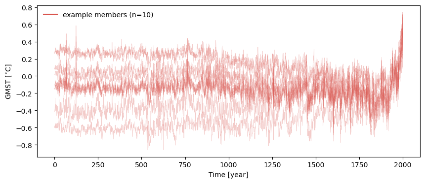
In some cases, it can be informative to look at a set of individual traces. By default, .plot_traces() plots ten traces, but it is simple enough to set num_traces to another choice value. The traces (however many) are chosen at random among the ensemble. Random number generators start from a seed number, so if it is important that the function yields the same plot each time it is rerun, set a value for seed (always an integer).
fig, ax = lmr_ens.plot_traces(seed=2110)
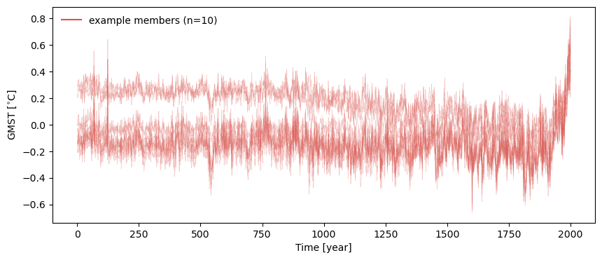
You can see it looks different with a seed of 42, despite the number’s cosmic importance.
fig, ax = lmr_ens.plot_traces(seed=42)
Plot envelope#
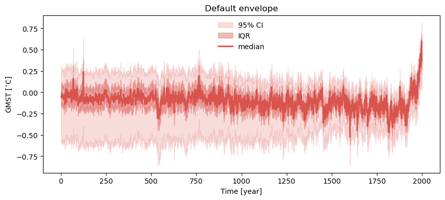
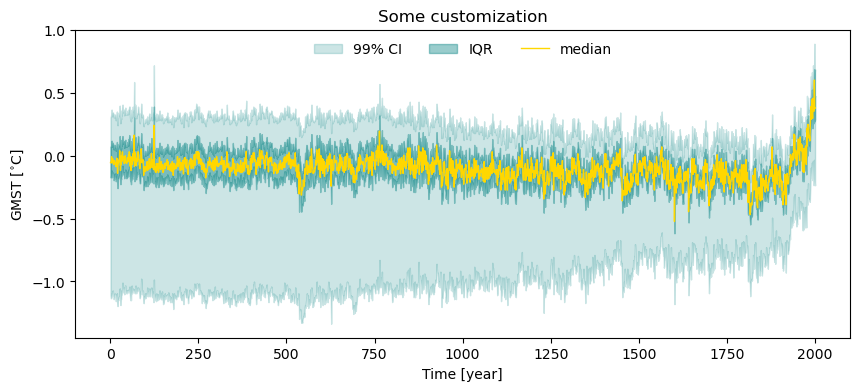
Instead of looking at the full set of traces, it can be useful to look at an envelope that highlights various features of the evolving distribution of the ensemble over time. By default, the quantiles displayed are [0.025, 0.25, 0.5, 0.75, 0.975], which means that it shows 95% confidence interval, the interquartile range (IQR), and the median. This plot can be customized for a different set of significance levels by passing a list of values to the parameter qs, in addition to various color, opacity, line style and label values.
lmr_ens.plot_envelope(title='Default envelope')
(<Figure size 1000x400 with 1 Axes>,
 <Axes: title={'center': 'Default envelope'}, xlabel='Time [year]', ylabel='GMST [$^{\\circ}$C]'>)
lmr_ens.plot_envelope(qs = [0.005, 0.25, 0.5, 0.75, 0.995], curve_lw=1,
                      shade_clr = 'teal', curve_clr='gold',
                      lgd_kwargs={'ncol':3,'loc':'upper center'},
                      outer_shade_label='99% CI', title='Some customization')
(<Figure size 1000x400 with 1 Axes>,
 <Axes: title={'center': 'Some customization'}, xlabel='Time [year]', ylabel='GMST [$^{\\circ}$C]'>)
Ensemble spectrum#
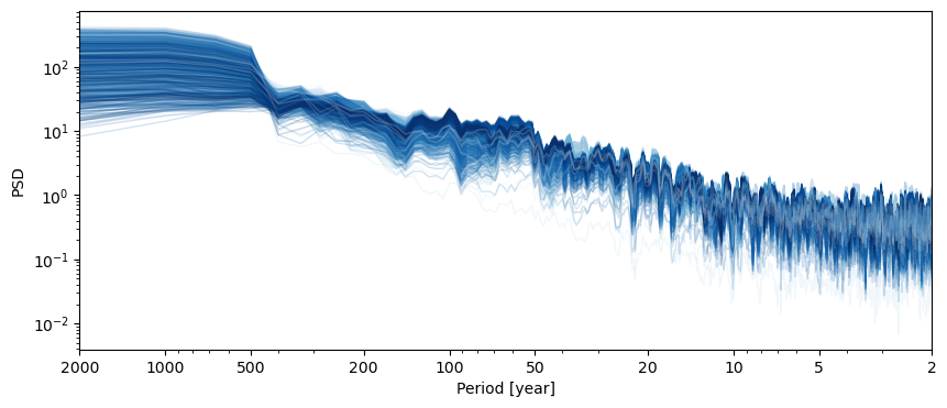
the beauty of such an object is that one can apply a complex workflow (e.g. spectral analysis) recursively with one command line. For instance, spectral analysis:
lmr_psd = lmr_ens.spectral(method='mtm')
Performing spectral analysis on individual series: 100%|██████████| 1000/1000 [00:11<00:00, 88.01it/s]
This is a MultiplePSD object, which has a dedicated plot() method working much like MultipleSeries.plot():
lmr_psd.plot(cmap='Blues',plot_kwargs={'linewidth':1,'alpha':0.2}, legend=False)
(<Figure size 1000x400 with 1 Axes>,
 <Axes: xlabel='Period [year]', ylabel='PSD'>)
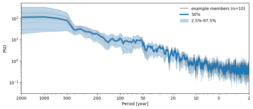
MultiplePSD objects also ships with a plot_envelope() function. This is really nifty if you’re trying to visualize a distribution of spectra obtained from an ensemble of series:
lmr_psd.plot_envelope(shade_clr = 'C0', curve_clr='C0')
(<Figure size 1000x400 with 1 Axes>,
 <Axes: xlabel='Period [year]', ylabel='PSD'>)
Plot distribution#
Some analysis methods assume that data have a normal distribution, so running .histplot() is a quick way to check whether this requirement is met for your EnsembleSeries.
fig, ax = lmr_ens.sel(time=slice(1257, 1260)).histplot()
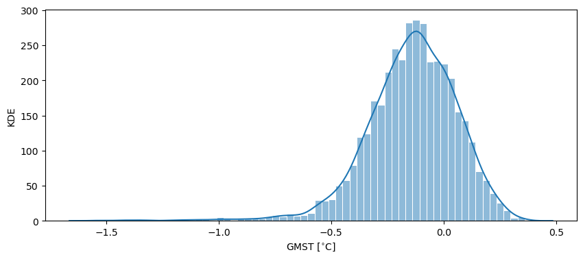
Notice how in this case we made use of the sel() method to select a specific time slice from the ensemble (in this case, years CE 1257 to 1260 inclusive).
%watermark -n -u -v -iv -w
Last updated: Thu, 12 Mar 2026

Python implementation: CPython
Python version       : 3.12.11
IPython version      : 9.6.0

pyleoclim: 1.3.1b0
pylipd   : 1.5.1
xarray   : 2025.12.0

Watermark: 2.6.0