
Working with GeoSeries#
Preamble#
The Series object, introduced here, is the entry point into the Pyleoclim universe, with very few metadata and a low bar to entry. However, geoscientific series, including paleoclimate timeseries, are often richer in information (particularly geolocation) that can be leveraged for further analysis. Therefore, we created a class called GeoSeries, which is a child of the Series object. As a child, GeoSeries inherits all the methods of its parent class as well as new methods that take advantage of the richer information.
Series properties that also apply to GeoSeries are as follows:
time: Time values for the time seriesvalue: Paleo values for the time seriestime_name(optional): Name of the time vector, (e.g., ‘Time’, ‘Age’). This is used to label the x-axis on plotstime_unit(optional): The units of the time axis (e.g., ‘years’)value_name(optional): The name of the paleo variable (e.g., ‘Temperature’)value_unit(optional): The units of the paleo variable (e.g., ‘deg C’)label(optional): Name of the time series (e.g., ‘Nino 3.4’)log(dict) – Dictionary of tuples documentating the various transformations applied to the objectkeep_log(bool) – Whether to keep a log of applied transformations. False by defaultimportedFrom(string) – source of the dataset. If it came from a LiPD file, this could be the datasetID propertyarchiveType(string) – climate archivedropna(bool) – Whether to drop NaNs from the series to prevent downstream functions from choking on them defaults to Truesort_ts(str) – Direction of sorting over the time coordinate; ‘ascending’ or ‘descending’ Defaults to ‘ascending’verbose(bool) – If True, will print warning messages if there is anyclean_ts(optional): set to True to remove the NaNs and make time axis strictly prograde with duplicated timestamps reduced by averaging the values Default is None.
In addition, GeoSeries includes the following properties:
lat(float): latitude (mandatory)lon(float): longitude (mandatory)elevation(float): elevationdepth(list): The values for the depth vectordepth_name(str): Name of the depth (e.g., top depth, mid-depth)depth_unit(str): The units for the depthsensorType(str): The type of sensor (e.g., foraminifera, buoys)observationType(str): The type of observations made (e.g., Mg/Ca, tree-ring width, )
As with the case with Series, the data can be ingested in different ways.
Goals:#
Create Pyleoclim Series objects from datasets stored as LiPD, NOAA txt files, and from PANGAEA.
Reading Time: 5 minutes
Keywords#
CSV; NetCDF; LiPD, Series; EnsembleSeries; MultipleSeries
Pre-requisites#
None. This tutorial assumes basic knowledge of Python. If you are not familiar with this coding language, check out this tutorial: http://linked.earth/LeapFROGS/.
Relevant Packages#
Pandas; Xarray; Pandas; Xarray; pylipd; pangaeapy
Data Description#
McCabe-Glynn, S., Johnson, K., Strong, C. et al. Variable North Pacific influence on drought in southwestern North America since AD 854. Nature Geosci 6, 617–621 (2013). doi:10.1038/ngeo1862
PAGES2k Consortium (Emile-Geay, J., McKay, N. et al): A global multiproxy database for temperature reconstructions of the Common Era. Sci Data 4, 170088 (2017). doi:10.1038/sdata.2017.88
Demonstration#
First we import our favorite packages:
%load_ext watermark

import pyleoclim as pyleo
from pylipd.lipd import LiPD
import pandas as pd
import numpy as np
LiPD#
For this demonstration, we will be reusing the same datasets and workflows as described here. But we will be instantiating GeoSeries instead of Series and looking at the extra functionalities that come with this new class.
Loading a single file#
data_path = '../data/Crystal.McCabe-Glynn.2013.lpd'
D = LiPD()
D.load(data_path)
Loading 1 LiPD files
100%|██████████| 1/1 [00:00<00:00, 5.73it/s]
Loaded..
df = D.get_timeseries_essentials(D.get_all_dataset_names()[0])
df
| dataSetName | archiveType | geo_meanLat | geo_meanLon | geo_meanElev | paleoData_variableName | paleoData_values | paleoData_units | paleoData_proxy | paleoData_proxyGeneral | time_variableName | time_values | time_units | depth_variableName | depth_values | depth_units | |
|---|---|---|---|---|---|---|---|---|---|---|---|---|---|---|---|---|
| 0 | Crystal.McCabe-Glynn.2013 | Speleothem | 36.59 | -118.82 | 1386.0 | d18o | [-8.01, -8.23, -8.61, -8.54, -8.6, -9.08, -8.9... | permil | None | None | age | [2007.7, 2007.0, 2006.3, 2005.6, 2004.9, 2004.... | yr AD | depth | [0.05, 0.1, 0.15, 0.2, 0.25, 0.3, 0.35, 0.4, 0... | mm |
Let’s have a look at the available metadata (column headers in the DataFrame):
df.columns
Index(['dataSetName', 'archiveType', 'geo_meanLat', 'geo_meanLon',
       'geo_meanElev', 'paleoData_variableName', 'paleoData_values',
       'paleoData_units', 'paleoData_proxy', 'paleoData_proxyGeneral',
       'time_variableName', 'time_values', 'time_units', 'depth_variableName',
       'depth_values', 'depth_units'],
      dtype='object')
From this, we can create a GeoSeries as follows:
metadata_dict={'time': df['time_values'].iloc[0],
              'value': df['paleoData_values'].iloc[0],
              'time_name': 'Time', 'label': df['dataSetName'].iloc[0],
              'time_unit': 'year CE',
              'value_name': df['paleoData_variableName'].iloc[0],
              'value_unit': df['paleoData_units'].iloc[0],
              'lat':df['geo_meanLat'].iloc[0],
              'lon':df['geo_meanLon'].iloc[0],
              'elevation': df['geo_meanElev'].iloc[0],
               'archiveType': df['archiveType'].iloc[0],
               'observationType': df['paleoData_proxy'].iloc[0],
               'auto_time_params':False
              }

ts = pyleo.GeoSeries(**metadata_dict)
Time axis values sorted in ascending order
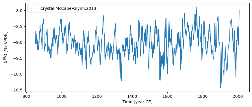
Let’s give this series better labels for better plots:
ts.value_name = '$\delta^{18}$O'
ts.value_unit = "‰ VPDB"
ts.plot()
(<Figure size 1000x400 with 1 Axes>,
 <Axes: xlabel='Time [year CE]', ylabel='$\\delta^{18}$O [‰ VPDB]'>)
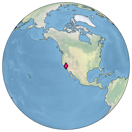
Additional methods enabled by GeoSeries currently involve mapping. For instance, let’s map the location of this record:
ts.map()
(<Figure size 1800x700 with 1 Axes>,
 {'map': <GeoAxes: xlabel='lon', ylabel='lat'>})

Let’s draw a thicker black edge around the symbol:
ts.map(edgecolor='black', scatter_kwargs ={'linewidth':2})
(<Figure size 1800x700 with 1 Axes>,
 {'map': <GeoAxes: xlabel='lon', ylabel='lat'>})
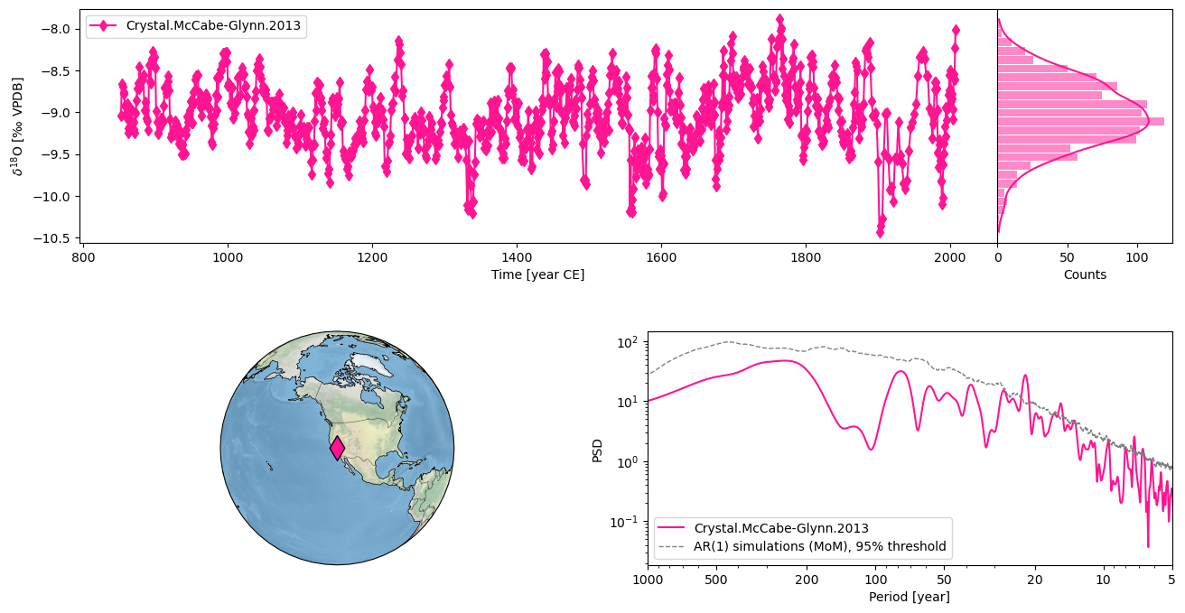
You can also create a dashboard summarizing the location of the record, plots the timeseries and runs spectral analysis to generate a periodogram:
ts.dashboard()
Using serial execution for this method on a Mac platform
Performing spectral analysis on individual series: 100%|██████████| 200/200 [00:39<00:00, 5.00it/s]
(<Figure size 1100x800 with 4 Axes>,
 {'ts': <Axes: xlabel='Time [year CE]', ylabel='$\\delta^{18}$O [‰ VPDB]'>,
  'dts': <Axes: xlabel='Counts'>,
  'map': {'map': <GeoAxes: xlabel='lon', ylabel='lat'>},
  'spec': <Axes: xlabel='Period [year]', ylabel='PSD'>})
MultipleGeoSeries#
Just like its parent class Series, GeoSeries can be bundled as well: MultipleGeoSeries has all the methods of MultipleGeoSeries plus some that are enabled by the additional metadata, particularly geolocation.
One can easily generate such objects by joining GeoSeries one by one, using the “&” method, as done in this example.
Here we show how to generate such an object by querying the LiPDGraph to obtain datasets from the PAGES2k database that are within the 20-60\(^{\circ}\) N band. In this we make use of the pylipd package, which will return everything in a pandas DataFrame. Note that this query is pointing towards an archive version of the database. To learn how to do queries to newer version of the database, see the pylipd tutorials.
import json
import requests
import io


url = 'https://linkedearth.graphdb.mint.isi.edu/repositories/LiPDVerse3'

query = """

PREFIX le: <http://linked.earth/ontology#>
PREFIX wgs: <http://www.w3.org/2003/01/geo/wgs84_pos#>

select ?val ?timeval ?varunits ?timeunits ?varname ?timevarname ?dsname ?lat ?lon ?alt ?archive ?proxy where {

    ?ds le:name ?dsname .
        OPTIONAL {?ds le:proxyArchiveType ?archive .}
    ?ds le:includesPaleoData ?data .

    ?ds le:collectedFrom ?loc .
    ?loc wgs:lat ?lat .
        FILTER(?lat<60 && ?lat>20)
    ?loc wgs:long ?lon .
    ?loc wgs:alt ?alt .

    ?data le:foundInMeasurementTable ?table .
    ?table le:includesVariable ?var .
    ?var le:name ?varname .
        FILTER regex(?varname, "temperature.*") .
    ?var le:hasValues ?val .
    ?var le:hasUnits ?varunits .
        VALUES ?varunits {"degC"} .
    ?var le:proxy ?proxy .
    ?var le:partOfCompilation ?comp .
    ?comp le:name "Pages2kTemperature" .


    ?table le:includesVariable ?timevar .
    ?timevar le:name ?timevarname .
        VALUES ?timevarname {"year"} .
    ?timevar le:hasValues ?timeval .
        OPTIONAL{?timevar le:hasUnits ?timeunits .}
}

"""

response = requests.post(url, data = {'query': query})

data = io.StringIO(response.text)
df = pd.read_csv(data, sep=",")

# Make list from the values string
df['val']=df['val'].apply(lambda row : np.fromstring(row.strip("[]"), sep=','))
df['timeval']=df['timeval'].apply(lambda row : np.fromstring(row.strip("[]"), sep=','))

df.head()
| val | timeval | varunits | timeunits | varname | timevarname | dsname | lat | lon | alt | archive | proxy | |
|---|---|---|---|---|---|---|---|---|---|---|---|---|
| 0 | [27.54, 26.67, 25.87, 27.78, 27.39, 26.98, 26.... | [1925.2, 1875.6, 1826.0, 1776.0, 1727.0, 1677.... | degC | AD | temperature | year | Ocn-DryTortugasA.Lund.2006 | 24.33 | -83.26 | -547.0 | marine sediment | foram Mg/Ca |
| 1 | [8.62, 8.41, 8.721341659, 8.800163059, 8.87029... | [1950.0, 1820.0, 1570.0, 1510.0, 1440.0, 1360.... | degC | AD | temperature | year | Ocn-EmeraldBasin.Keigwin.2007 | 43.53 | -62.48 | -250.0 | marine sediment | alkenone |
| 2 | [20.4, 20.4, 20.7, 20.6, 20.5, 20.2, 19.3, 19.... | [1950.0, 1937.0, 1924.0, 1911.0, 1898.0, 1886.... | degC | AD | temperature | year | NAm-DarkLake.Gajewski.1988 | 45.30 | -91.50 | 334.0 | lake sediment | pollen |
| 3 | [-7.1, nan, -6.3, -4.5, -6.4, -7.8, -5.7, -5.3... | [1500.0, 1501.0, 1502.0, 1503.0, 1504.0, 1505.... | degC | AD | temperature | year | Eur-Tallinn.Tarand.2001 | 59.40 | 24.75 | 10.0 | documents | historic |
| 4 | [8.84, 8.6, 9.32, 9.99, 9.78, 9.88, 10.06, 9.7... | [1950.0, 1942.06, 1934.12, 1926.19, 1918.25, 1... | degC | AD | temperature | year | Ocn-EmeraldBasin.Keigwin.2003 | 45.89 | -62.80 | -250.0 | marine sediment | alkenone |
Next, we iterate over the rows, put the relevant information into the right place of a list GeoSeries objects:
ts_list = []
for _, row in df.iterrows():
    ts_list.append(pyleo.GeoSeries(time=row['timeval'],value=row['val'],
                            time_name='Year',value_name=row['varname'],
                            time_unit=row['timeunits'], value_unit=row['varunits'],
                            lat = row['lat'], lon = row['lon'],
                            elevation = row['alt'],
                            archiveType = row['archive'],
                            observationType=row['proxy'],
                            label=row['dsname']+'_'+row['proxy'], verbose = False))
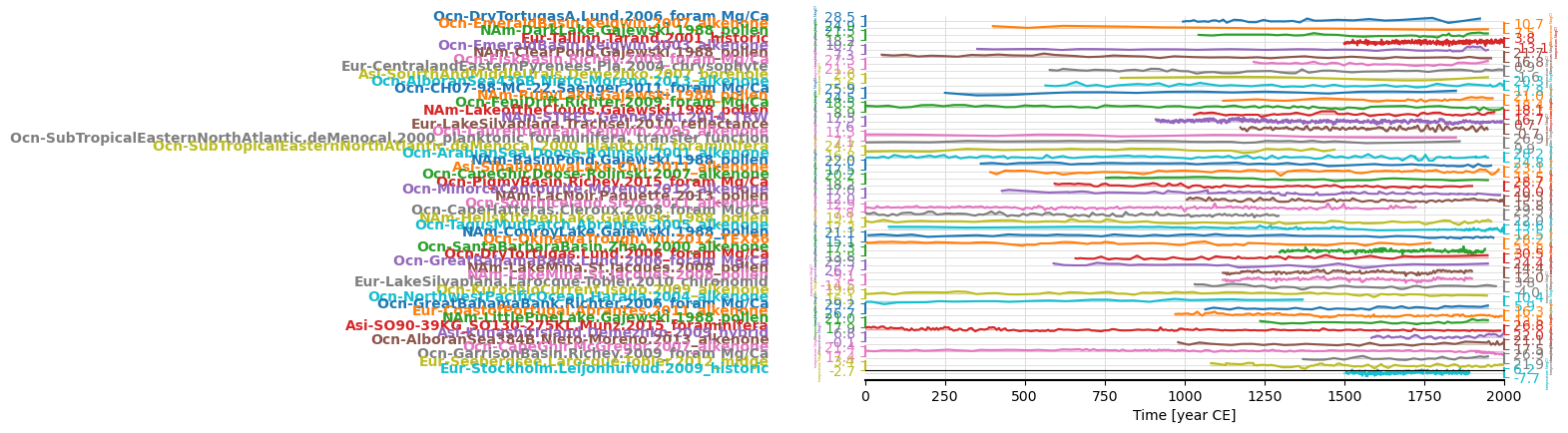
Finally, we instantiate a MultipleGeoSeries out of this, and make sure to harmonize all the time units for ease of plotting:
pages2k = pyleo.MultipleGeoSeries(ts_list,time_unit='year CE')
pages2k.stackplot(ylabel_fontsize=2, xlim=[0,2000])
(<Figure size 640x480 with 51 Axes>,
 {0: <Axes: ylabel='temperature [degC]'>,
  1: <Axes: ylabel='temperature [degC]'>,
  2: <Axes: ylabel='temperature [degC]'>,
  3: <Axes: ylabel='temperature [degC]'>,
  4: <Axes: ylabel='temperature [degC]'>,
  5: <Axes: ylabel='temperature [degC]'>,
  6: <Axes: ylabel='temperature [degC]'>,
  7: <Axes: ylabel='temperature [degC]'>,
  8: <Axes: ylabel='temperature [degC]'>,
  9: <Axes: ylabel='temperature [degC]'>,
  10: <Axes: ylabel='temperature [degC]'>,
  11: <Axes: ylabel='temperature [degC]'>,
  12: <Axes: ylabel='temperature [degC]'>,
  13: <Axes: ylabel='temperature [degC]'>,
  14: <Axes: ylabel='temperature [degC]'>,
  15: <Axes: ylabel='temperature [degC]'>,
  16: <Axes: ylabel='temperature [degC]'>,
  17: <Axes: ylabel='temperature [degC]'>,
  18: <Axes: ylabel='temperature [degC]'>,
  19: <Axes: ylabel='temperature [degC]'>,
  20: <Axes: ylabel='temperature [degC]'>,
  21: <Axes: ylabel='temperature [degC]'>,
  22: <Axes: ylabel='temperature [degC]'>,
  23: <Axes: ylabel='temperature [degC]'>,
  24: <Axes: ylabel='temperature [degC]'>,
  25: <Axes: ylabel='temperature [degC]'>,
  26: <Axes: ylabel='temperature [degC]'>,
  27: <Axes: ylabel='temperature [degC]'>,
  28: <Axes: ylabel='temperature [degC]'>,
  29: <Axes: ylabel='temperature [degC]'>,
  30: <Axes: ylabel='temperature [degC]'>,
  31: <Axes: ylabel='temperature [degC]'>,
  32: <Axes: ylabel='temperature [degC]'>,
  33: <Axes: ylabel='temperature [degC]'>,
  34: <Axes: ylabel='temperature [degC]'>,
  35: <Axes: ylabel='temperature [degC]'>,
  36: <Axes: ylabel='temperature [degC]'>,
  37: <Axes: ylabel='temperature [degC]'>,
  38: <Axes: ylabel='temperature [degC]'>,
  39: <Axes: ylabel='temperature [degC]'>,
  40: <Axes: ylabel='temperature [degC]'>,
  41: <Axes: ylabel='temperature [degC]'>,
  42: <Axes: ylabel='temperature [degC]'>,
  43: <Axes: ylabel='temperature [degC]'>,
  44: <Axes: ylabel='temperature [degC]'>,
  45: <Axes: ylabel='temperature [degC]'>,
  46: <Axes: ylabel='temperature [degC]'>,
  47: <Axes: ylabel='temperature [degC]'>,
  48: <Axes: ylabel='temperature [degC]'>,
  49: <Axes: ylabel='temperature [degC]'>,
  'x_axis': <Axes: xlabel='Time [year CE]'>})
Mapping collections#
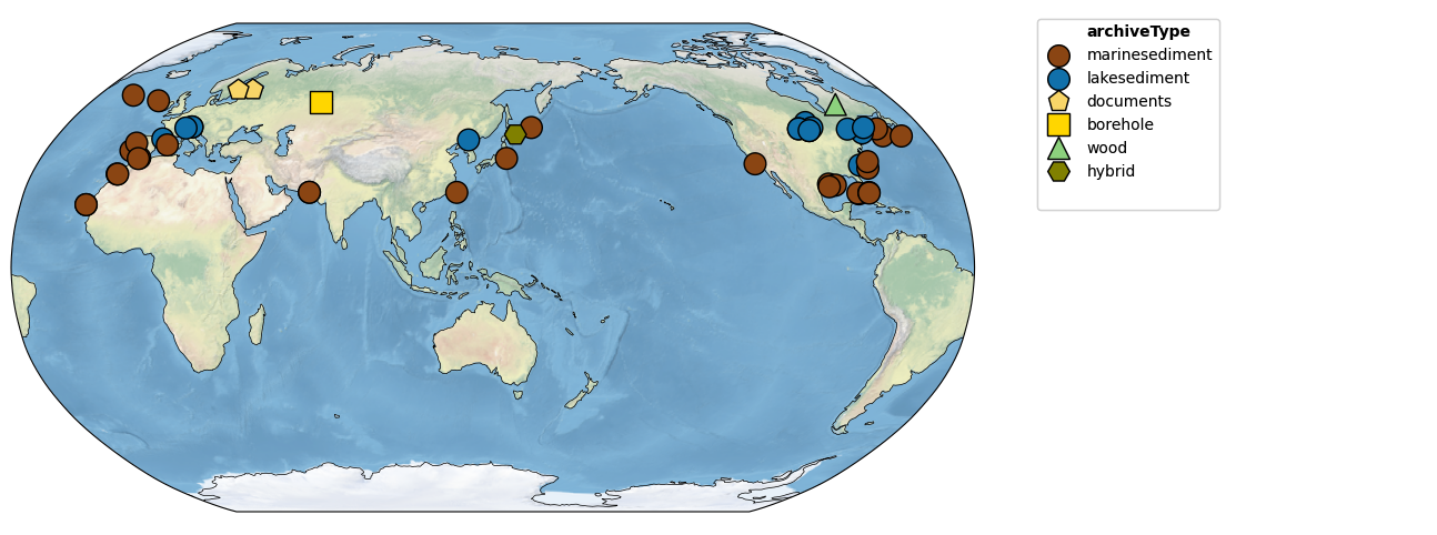
The first thing one might do is map those records:
pages2k.map()
(<Figure size 1800x600 with 2 Axes>,
 {'map': <GeoAxes: xlabel='lon', ylabel='lat'>, 'leg': <Axes: >})
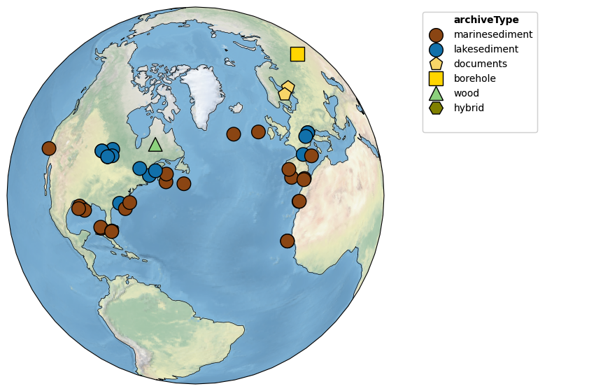
Let’s say we wanted to focus on those parts of PAGES2k in North America; you could focus the map in this way, and use a more appropriate projection:
NA_coord = {'central_latitude':40, 'central_longitude':-50}
pages2k.map(projection='Orthographic',proj_default=NA_coord)
(<Figure size 1800x700 with 2 Axes>,
 {'map': <GeoAxes: xlabel='lon', ylabel='lat'>, 'leg': <Axes: >})
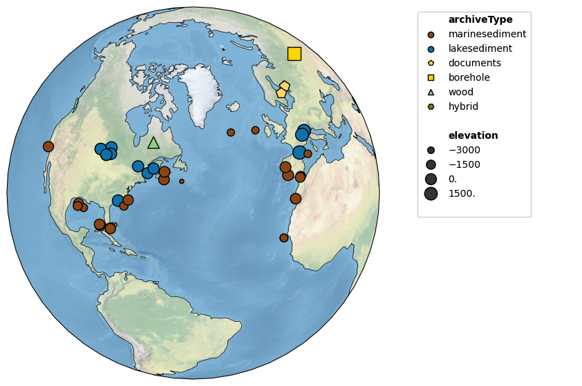
By default, the shape and colors of symbols denote proxy archives; however, one can use either graphical device to convey other information. For instance, if elevation is available, it may be displayed by size, like so:
pages2k.map(projection='Orthographic', size='elevation', proj_default=NA_coord)
(<Figure size 1800x700 with 2 Axes>,
 {'map': <GeoAxes: xlabel='lon', ylabel='lat'>, 'leg': <Axes: >})
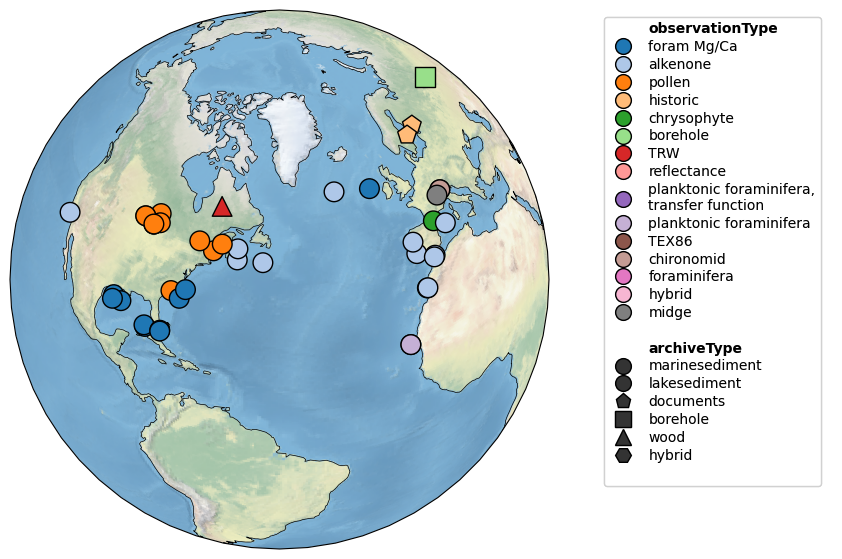
Same with observationType:
pages2k.map(projection='Orthographic', hue = 'observationType', proj_default=NA_coord)
(<Figure size 1800x700 with 2 Axes>,
 {'map': <GeoAxes: xlabel='lon', ylabel='lat'>, 'leg': <Axes: >})
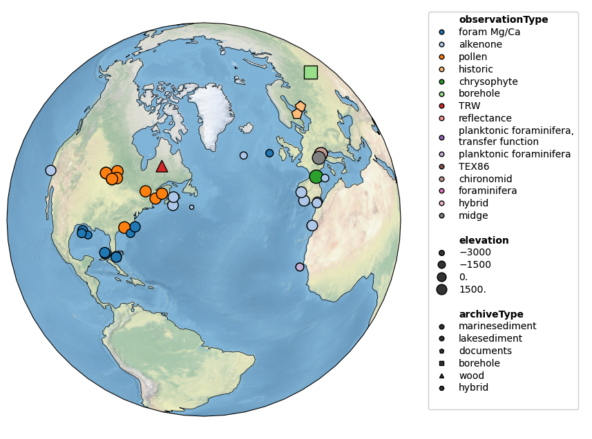
All three sources of information may be combined, but the figure height then needs to be enlarged manually to fit the legend. This is done via the figsize argument:
pages2k.map(projection='Orthographic',hue='observationType',
                       size='elevation', proj_default=NA_coord, figsize=[18, 8])
(<Figure size 1800x800 with 2 Axes>,
 {'map': <GeoAxes: xlabel='lon', ylabel='lat'>, 'leg': <Axes: >})
Mapping Neighbors#
Let’s return to our Crystal Cave example. How many PAGES2k records identified above lie within a certain radius of this cave? That is easy to map:
ts.map_neighbors(pages2k)
(<Figure size 1800x700 with 2 Axes>,
 {'map': <GeoAxes: xlabel='lon', ylabel='lat'>, 'leg': <Axes: >})
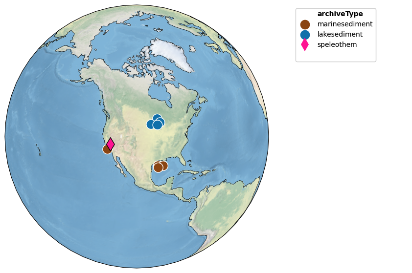
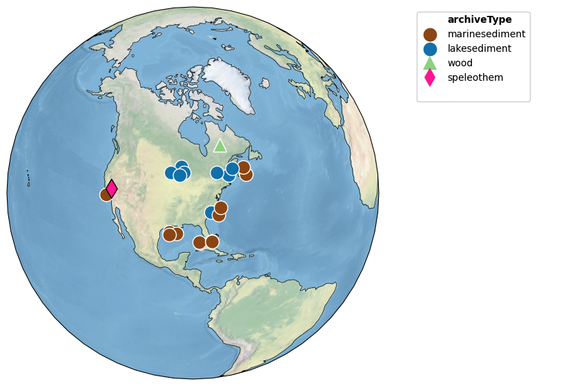
Note how the target record (here, Crystal Cave) is outlined in black, while all the other ones are outlined in white. It is easy to widen the search radius to include more records:
ts.map_neighbors(pages2k, radius=5000)
(<Figure size 1800x700 with 2 Axes>,
 {'map': <GeoAxes: xlabel='lon', ylabel='lat'>, 'leg': <Axes: >})
For examples of actual data analysis using MultipleGeoSeries and MulEnsGeoSeries, see the tutorial on Principal Component Analysis.
%watermark -n -u -v -iv -w
Last updated: Thu, 12 Mar 2026

Python implementation: CPython
Python version       : 3.12.11
IPython version      : 9.6.0

json     : 2.0.9
numpy    : 2.3.3
pandas   : 2.3.3
pyleoclim: 1.3.1b0
pylipd   : 1.5.1
requests : 2.32.5

Watermark: 2.6.0