Correlation Analysis in Pyleoclim

by Julien Emile-Geay

Preamble

This tutorial has two parts, highlighting two important applications of correlation analysis to paleoclimatology.

1. The first tackles the comparison of age-uncertain records, and is inspired by a similar one in Pyleoclim’s sister package, GeoChronR.

2. The second shows how to compute correlations between a record and a gridded field, illustrative of the multiple comparisons (aka “Look Elsewhere”) effect.

We also show how the latest Pyleoclim version can apply different types of surrogates for significance testing, and compute different metrics of association, from the usual Pearson correlation to more exotic statistics like Spearman’s \(\rho\) or Kendall’s \(\tau\), which sidestep the assumption of a linear relationship between series.

Goals:

• load and create age ensemble data

• run correlation workflow on those ensembles, using various statistics and surrogates

• interpret the results of these correlation tests, especially when multiple tests are carried out at once

• go between LiPD-formatted paleo data and Xarray datasets, using pandas and Pyleoclim as go-betweens

Reading Time:

10 minutes

Keywords

Age ensembles, Surogates, multiple hypotheses, serial correlation, significance

Pre-requisites

None. This tutorial assumes basic knowledge of Python. If you are not familiar with this coding language, check out this tutorial: http://linked.earth/LeapFROGS/.

Relevant Packages

Pickle, Pyleoclim

Data Description

• Hulu Cave record: https://www.science.org/doi/10.1126/science.1064618

• GISP2: https://icecores.org/inventory/gisp2

• ERSSTv5: Huang et al, (2017)

• Palmyra modern Sr/Ca data: Nurhati et al (2011)

Let’s import the packages needed for this tutorial:

%load_ext watermark
import pickle
import pyleoclim as pyleo

Age-uncertain Correlations

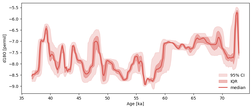
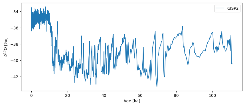
This example compares two high-resolution paleoclimate records with quantifiable age uncertainties: the Hulu Cave speleothem record of Wang et al. (2001) and the GISP2 ice core record. Both measure stable oxygen isotopes (\(\delta^{18} \mathrm{O}\)), though these proxy systems have radically different interpretations, which are not relevant here.

On multi-millennial timescales, the two datasets display such similar features that the well-dated Hulu Cave record has been used to argue for atmospheric teleconnections between the regions and support the independent chronology of GISP2. In this example, we revisit this relation quantitatively and use their age models (one provided, one created using a built-in Pyleoclim function), to calculate the impact of age uncertainty on the correlation between these two iconic datasets.

First, let’s look at the Hulu Cave dataset from Wang et al. (2001), with age ensemble generates using BChron:

with open('../data/hulu_ensemble.pkl','rb') as handle:
    Hulu = pickle.load(handle)
Hulu.label = 'Hulu Cave'
Hulu.value_name = r'$\delta^{18} \mathrm{O}$'
Hulu.value_unit = '‰'
Hulu = Hulu.convert_time_unit('ky BP')
Hulu.common_time().plot_envelope()

(<Figure size 1000x400 with 1 Axes>,
 <Axes: xlabel='Age [ka]', ylabel='d18O [permil]'>)

Next we load GISP2, which actually ships with Pyleoclim (see this tutorial). Its original time unit is “years BP”, which we convert to “ky BP” (thousands of years before present) to harmonize with Hulu:

GISP2 = pyleo.utils.load_dataset('GISP2')
GISP2 = GISP2.convert_time_unit('ky BP')
GISP2.plot()

(<Figure size 1000x400 with 1 Axes>,
 <Axes: xlabel='Age [ka]', ylabel='$\\delta^{18} \\mathrm{O}$ [‰]'>)

Create age ensemble

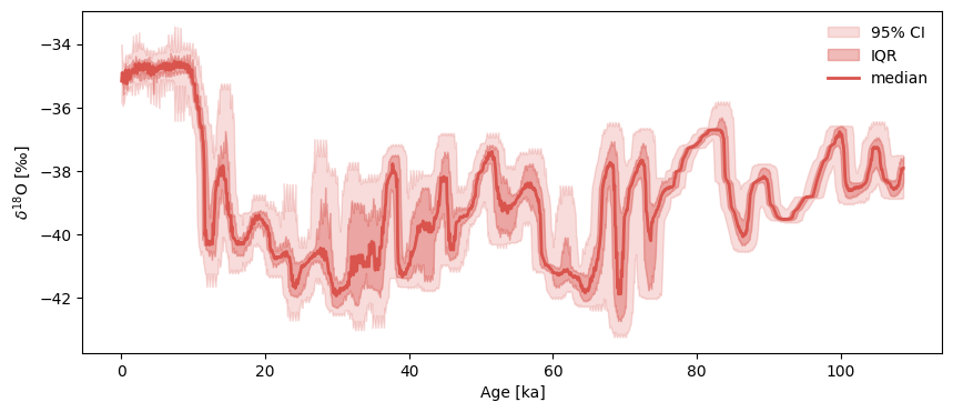
Hulu already has an age ensemble, but GISP2 doesn’t. To generate a plausible one, we use a Pyleoclim function called random_time_axis to create a 1000-member EnsembleSeries object with time perturbations of \(\pm100y\) with a 2% probability:

nEns = 1000
n = len(GISP2.time)
slist = []
for _ in range(nEns):
    pert = pyleo.utils.tsmodel.random_time_axis(n,
                                         delta_t_dist='random_choice',
                                         param =[[-0.1,0,0.1],[0.02,0.96,0.02]])
    ts = GISP2.copy()
    ts.time = GISP2.time + pert
    slist.append(ts)
GISP2e = pyleo.EnsembleSeries(slist)

Notice how we specified parameters here: param =[[-0.1,0,0.1],[0.02,0.96,0.02]] means that the time increment perturbations (departures from 1), are rare and symmetric, being 0ky 96% of the time, and \(\pm0.1\)ky the remaining 4% of the time. Let us plot the result:

GISP2e.common_time().plot_envelope()

(<Figure size 1000x400 with 1 Axes>,
 <Axes: xlabel='Age [ka]', ylabel='$\\delta^{18} \\mathrm{O}$ [‰]'>)

Correlating the medians

Before delving into the ensembles, let’s extract their medians and explore their correlation, to showcase a few of Pyleoclim’s capabilities. The default measure of association is Pearson’s product-moment correlation, more commonly known as Pearson’s R. However, there are several ways of assessing the significance of the result. We use 3 here:

• the built-in test from SciPy

• a Monte Carlo simulation using AR(1) surrogates.

• a Monte Carlo simulation using phase-randomized surrogates

Effect of persistence

Hulu_m = Hulu.common_time().quantiles(qs=[0.5]).series_list[0] # this turns it into a Series
GISP2_m = GISP2e.common_time().quantiles(qs=[0.5]).series_list[0] # this turns it into a Series
for method in ['built-in','ar1sim','phaseran',]:
    corr_m = Hulu_m.correlation(GISP2_m,method=method)
    print(corr_m)

  statistic    critical value  p-value    signif. (α: 0.05)
-----------  ----------------  ---------  -------------------
  -0.395784               nan  < 1e-13    True

Evaluating association on surrogate pairs: 100%|██████████| 1000/1000 [00:00<00:00, 1523.52it/s]

  statistic    critical value    p-value  signif. (α: 0.05)
-----------  ----------------  ---------  -------------------
  -0.395784         -0.507637       0.23  False

Evaluating association on surrogate pairs: 100%|██████████| 1000/1000 [00:00<00:00, 1618.51it/s]

  statistic    critical value    p-value  signif. (α: 0.05)
-----------  ----------------  ---------  -------------------
  -0.395784         -0.369923        0.1  False

type(corr_m)

pyleoclim.core.corr.Corr

The result of these calculations is stored in a Corr object, which contains several things:

• r (float), the statistic measuring association

• r_crit (float), the critical value of this statistic (i.e. the threshold value that must be exceeded (in absolute value) to call this “significant”). This is provided as a convenience for some applications, and cannot be computed in all cases (e.g. the built-in method)

• p (float), the p-value, which is used to decide whether the correlation is in any way remarkable (“significant”)

• signif, a boolean indicating whether significance was reached, at the indicated level (0.05 by default)

We see that the three methods return the same value \(r \approx -0.4\) but quite different assessments of the \(p\)-value:

• the built-in test, which assumes that the data are Gaussian and IID, suggests a highly significant result, with a p-value less than \(10^{-13}\).

• the test against both surrogates suggests the correlation is not significant at the 95% level.

This is a reminder of the importance of judiciously applying statistical tests in the paleo context. As recounted by Hu et al (2017), there are 3 major pitfalls for paleo-correlations. The first, which is here on full display, is that serial correlation (persistence) undermines the assumption that consecutive samples are independent, thereby radically reducing the number of degrees of freedom available to the test. This can often invalidate such tests entirely. Accordingly, Pyleoclim implements a modified version of the built-in test, which estimates the effective degrees of freedom \(n_\mathrm{eff}\) lost to serial correlation. This method is available as ttest, but in this case it would not work because it results in \(n_\mathrm{eff}<10\), which is too small for this test to make any sense (try it!).

Effect of nonlinearity

Now we showcase how to apply a different statistic, for example, Spearman’s \(\rho\) and Kendall’s \(\tau\):

for method in ['built-in','ar1sim','phaseran']:
    corr_s = Hulu_m.correlation(GISP2_m,statistic='spearmanr',method=method)
    print(corr_s)

  statistic    critical value  p-value    signif. (α: 0.05)
-----------  ----------------  ---------  -------------------
  -0.396495               nan  < 1e-13    True

Evaluating association on surrogate pairs: 100%|██████████| 1000/1000 [00:00<00:00, 1016.97it/s]

  statistic    critical value    p-value  signif. (α: 0.05)
-----------  ----------------  ---------  -------------------
  -0.396495         -0.515154        0.2  False

Evaluating association on surrogate pairs: 100%|██████████| 1000/1000 [00:00<00:00, 1023.54it/s]

  statistic    critical value    p-value  signif. (α: 0.05)
-----------  ----------------  ---------  -------------------
  -0.396495          -0.37607       0.07  False

Same for Kendall’s \(\tau\):

for method in ['built-in','ar1sim','phaseran']:
    corr_t = Hulu_m.correlation(GISP2_m,statistic='kendalltau',method=method)
    print(corr_t)

  correlation  p-value    signif. (α: 0.05)
-------------  ---------  -------------------
    -0.263541  < 1e-12    True

Evaluating association on surrogate pairs: 100%|██████████| 1000/1000 [00:00<00:00, 2598.87it/s]

  correlation    p-value  signif. (α: 0.05)
-------------  ---------  -------------------
    -0.263541       0.23  False

Evaluating association on surrogate pairs: 100%|██████████| 1000/1000 [00:00<00:00, 2885.02it/s]

  correlation    p-value  signif. (α: 0.05)
-------------  ---------  -------------------
    -0.263541       0.08  False

We see that Spearman’s \(\rho\) yields results very close to Pearson’s \(r\) (the phase randomization test is now at the edge of significance), so nonlinearity is probably not a main concern. Quantitatively, Kendall’s \(\tau\) estimates a lower absolute correlation, but assessments of significance are the same as before: the built-in test suggests a highly significant correlation, a result contradicted by the surrogates. All in all, a reasonable investigator would dismiss this correlation between median age models as non significant.

Multiple Comparison

We now tackle the multiple comparisons problem, which can create the appearance of significant results because, at the 5% level, 5% of tests will return a false positive, so if thousands of comparisons are carried out (as is the case here), then one expects that a few dozen of them will be identified as “significant” at that level (\(\alpha=0.05\)). A solution to this problem was worked out in 1995 as the false-discovery rate procedure (FDR), which is implemented in Pyleoclim.

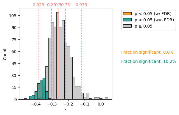
The latter can carry out correlations between EnsembleSeries objects, and here the result has more features. This calculation, using 1000 surrogates for each of the 1000 age models, computes a million correlations, and therefore takes a few minutes:

corr_e = Hulu.correlation(GISP2e, method='phaseran',number=1000)

Looping over 1000 Series in the ensemble

  0%|          | 0/1000 [00:00<?, ?it/s]

Time axis values sorted in ascending order

100%|██████████| 1000/1000 [13:22<00:00,  1.25it/s]

corr_e.plot()

(<Figure size 400x400 with 1 Axes>, <Axes: xlabel='$r$', ylabel='Count'>)

type(corr_e)

pyleoclim.core.correns.CorrEns

Whereas the previous correlation results were stored in a Corr object, this one is stored in a CorrEns object. It contains very similar information to Corr, but the lists can be tedious to inspect in print, so a visual inspection via its plot() method (see figure above) is far more useful.

It shows that :

• the vast majority of correlations between individual ensemble members are judged non-significant.

• a subset of those (around 9%) are found significant. However, when accounting for the multiple comparisons problem via FDR, none of them are found significant.

This confirms what was found earlier using median age models. This is not always the case, as the median (or mean) is often a very poor summary of a dataset. When ensembles are available, it is always preferable to look at them in their entirety, something Pyleoclim makes practical.

Field Correlations

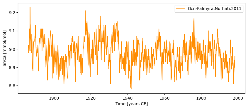
Another example of multiple comparison arises when assessing correlations between a single series (e.g. a paleoclimate record, or an instrumental station) and an instrumental climate field. Here, we use as our record the coral Sr/Ca series (a proxy for sea-surface temperature) from Nurhati et al (2011). The data are from Palmyra Island in the tropical Pacific, at the edge of the NINO3.4 box (a popular measure of the state of El Niño Southern Oscillation). We compare it to the sea-surface temperature analysis of ERSSTv5 (Huang et al, 2017).

To do so we leverage the wonderful Xarray package to load the data directly from NCEI’s servers so they never have to be explicitly downloaded (aka “lazy-loading”). We also make use of pyLiPD and a few other packages.

from pylipd.lipd import LiPD
import xarray as xr
import matplotlib.pyplot as plt
import cartopy.crs as ccrs
import numpy as np

D = LiPD()
D.load('../data/Ocn-Palmyra.Nurhati.2011.lpd')
timeseries,df = D.get_timeseries(D.get_all_dataset_names(),to_dataframe=True)
df

Loading 1 LiPD files

100%|██████████| 1/1 [00:00<00:00, 28.56it/s]

Loaded..
Extracting timeseries from dataset: Ocn-Palmyra.Nurhati.2011 ...

	mode	time_id	studyName	originalDataURL	hasUrl	pub1_author	pub1_url	pub1_institution	pub1_urldate	pub1_citeKey	...	paleoData_values	paleoData_proxyObservationType	paleoData_sensorGenus	paleoData_useInGlobalTemperatureAnalysis	paleoData_notes	paleoData_sensorSpecies	paleoData_proxy	paleoData_compilation_nest	paleoData_interpretation	paleoData_inCompilation
0	paleoData	age	Nurhati2011_Palmyra	http://hurricane.ncdc.noaa.gov/pls/paleox/f?p=...	https://data.mint.isi.edu/files/lipd/Ocn-Palmy...	I.S. Nurhati	[https://www.ncdc.noaa.gov/paleo/study/8609]	World Data Center for Paleoclimatology	2010.0	nurhati2010httpswwwncdcnoaagovpaleostudy8609Da...	...	[1998.21, 1998.13, 1998.04, 1997.96, 1997.88, ...	NaN	NaN	NaN	NaN	NaN	NaN	NaN	NaN	NaN
1	paleoData	age	Nurhati2011_Palmyra	http://hurricane.ncdc.noaa.gov/pls/paleox/f?p=...	https://data.mint.isi.edu/files/lipd/Ocn-Palmy...	I.S. Nurhati	[https://www.ncdc.noaa.gov/paleo/study/8609]	World Data Center for Paleoclimatology	2010.0	nurhati2010httpswwwncdcnoaagovpaleostudy8609Da...	...	[0.39, 0.35, 0.35, 0.35, 0.36, 0.22, 0.33, 0.3...	d18O	Porites	False	d18Osw (residuals calculated from coupled SrCa...	lutea	d18O	NaN	NaN	NaN
2	paleoData	age	Nurhati2011_Palmyra	http://hurricane.ncdc.noaa.gov/pls/paleox/f?p=...	https://data.mint.isi.edu/files/lipd/Ocn-Palmy...	I.S. Nurhati	[https://www.ncdc.noaa.gov/paleo/study/8609]	World Data Center for Paleoclimatology	2010.0	nurhati2010httpswwwncdcnoaagovpaleostudy8609Da...	...	[8.96, 8.9, 8.91, 8.94, 8.92, 8.89, 8.87, 8.81...	Sr/Ca	Porites	True	; paleoData_variableName changed - was origina...	lutea	Sr/Ca	MNE, NJA	[{'scope': 'climate', 'direction': 'negative',...	Ocean2k_v1.0.0
3	paleoData	age	Nurhati2011_Palmyra	http://hurricane.ncdc.noaa.gov/pls/paleox/f?p=...	https://data.mint.isi.edu/files/lipd/Ocn-Palmy...	I.S. Nurhati	[https://www.ncdc.noaa.gov/paleo/study/8609]	World Data Center for Paleoclimatology	2010.0	nurhati2010httpswwwncdcnoaagovpaleostudy8609Da...	...	[1998.29, 1998.21, 1998.13, 1998.04, 1997.96, ...	NaN	NaN	NaN	NaN	NaN	NaN	NaN	NaN	NaN
4	paleoData	age	Nurhati2011_Palmyra	http://hurricane.ncdc.noaa.gov/pls/paleox/f?p=...	https://data.mint.isi.edu/files/lipd/Ocn-Palmy...	I.S. Nurhati	[https://www.ncdc.noaa.gov/paleo/study/8609]	World Data Center for Paleoclimatology	2010.0	nurhati2010httpswwwncdcnoaagovpaleostudy8609Da...	...	[-5.41, -5.47, -5.49, -5.43, -5.48, -5.53, -5....	d18O	Porites	False	Duplicate of modern d18O record presented in C...	lutea	d18O	MNE, NJA	[{'direction': 'negative', 'hasVariable': {'la...	NaN

5 rows × 90 columns

Let’s put the Sr/Ca data into a GeoSeries object so we can easily plot it in space and time:

row = df[df['paleoData_variableName']=='Sr/Ca']

srca = pyleo.GeoSeries(
    time=row['year'].values[0],
    value=row['paleoData_values'].values[0],
    lon = df['geo_meanLon'][0],
    lat = df['geo_meanLat'][0],
    archiveType = 'coral',
    time_name = 'Time',
    time_unit = 'years CE',
    value_name = 'Sr/Ca',
    value_unit = row['paleoData_units'].values[0],
    label='Ocn-Palmyra.Nurhati.2011',
    auto_time_params = False,
) # load only the Sr/Ca observations
srca.plot()

Time axis values sorted in ascending order

(<Figure size 1000x400 with 1 Axes>,
 <Axes: xlabel='Time [years CE]', ylabel='Sr/Ca [mmol/mol]'>)

srca.map()

(<Figure size 1800x700 with 1 Axes>,
 {'map': <GeoAxes: xlabel='lon', ylabel='lat'>})

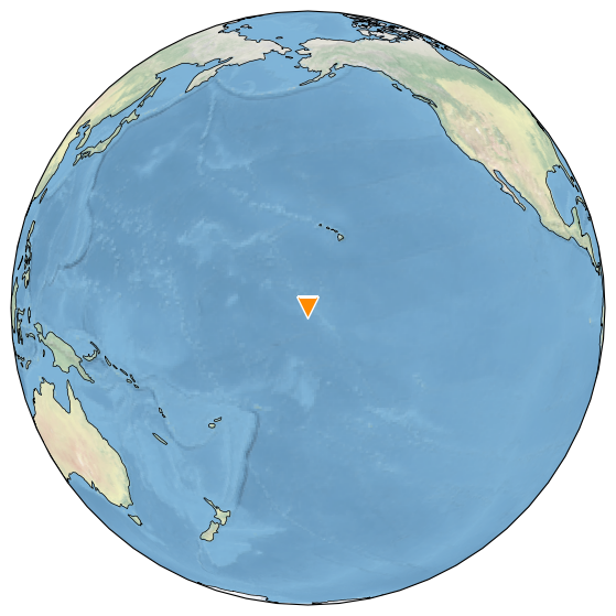
Palmyra Island sits in the very central Pacific, and we expect to see large-scale correlations with SST data.

Next we load the ERSSTv5 dataset. Note that the actual dat are not being transferred over the network yet; all we are getting is a pointer towards a netCDF file on a NOAA THREDDS server. The real crunching will come later.

filepath = 'https://psl.noaa.gov/thredds/dodsC/Datasets/noaa.ersst.v5/sst.mnmean.nc'
ersstv5 = xr.open_dataset(filepath)
ersstv5

<xarray.Dataset>
Dimensions:    (lat: 89, lon: 180, time: 2052, nbnds: 2)
Coordinates:
  * lat        (lat) float32 88.0 86.0 84.0 82.0 ... -82.0 -84.0 -86.0 -88.0
  * lon        (lon) float32 0.0 2.0 4.0 6.0 8.0 ... 352.0 354.0 356.0 358.0
  * time       (time) datetime64[ns] 1854-01-01 1854-02-01 ... 2024-12-01
Dimensions without coordinates: nbnds
Data variables:
    time_bnds  (time, nbnds) float64 ...
    sst        (time, lat, lon) float32 ...
Attributes: (12/39)
    climatology:                     Climatology is based on 1971-2000 SST, X...
    description:                     In situ data: ICOADS2.5 before 2007 and ...
    keywords_vocabulary:             NASA Global Change Master Directory (GCM...
    keywords:                        Earth Science > Oceans > Ocean Temperatu...
    instrument:                      Conventional thermometers
    source_comment:                  SSTs were observed by conventional therm...
    ...                              ...
    comment:                         SSTs were observed by conventional therm...
    summary:                         ERSST.v5 is developed based on v4 after ...
    dataset_title:                   NOAA Extended Reconstructed SST V5
    _NCProperties:                   version=2,netcdf=4.6.3,hdf5=1.10.5
    data_modified:                   2025-01-03
    DODS_EXTRA.Unlimited_Dimension:  time

xarray.Dataset

• Dimensions:
  • lat: 89
  • lon: 180
  • time: 2052
  • nbnds: 2
• Coordinates: (3)
  • lat
    (lat)
    float32
    88.0 86.0 84.0 ... -86.0 -88.0

    units :

    degrees_north

    long_name :

    Latitude

    actual_range :

    [ 88. -88.]

    standard_name :

    latitude

    axis :

    Y

    coordinate_defines :

    center

    array([ 88.,  86.,  84.,  82.,  80.,  78.,  76.,  74.,  72.,  70.,  68.,  66.,
            64.,  62.,  60.,  58.,  56.,  54.,  52.,  50.,  48.,  46.,  44.,  42.,
            40.,  38.,  36.,  34.,  32.,  30.,  28.,  26.,  24.,  22.,  20.,  18.,
            16.,  14.,  12.,  10.,   8.,   6.,   4.,   2.,   0.,  -2.,  -4.,  -6.,
            -8., -10., -12., -14., -16., -18., -20., -22., -24., -26., -28., -30.,
           -32., -34., -36., -38., -40., -42., -44., -46., -48., -50., -52., -54.,
           -56., -58., -60., -62., -64., -66., -68., -70., -72., -74., -76., -78.,
           -80., -82., -84., -86., -88.], dtype=float32)

  • lon
    (lon)
    float32
    0.0 2.0 4.0 ... 354.0 356.0 358.0

    units :

    degrees_east

    long_name :

    Longitude

    actual_range :

    [ 0. 358.]

    standard_name :

    longitude

    axis :

    X

    coordinate_defines :

    center

    array([  0.,   2.,   4.,   6.,   8.,  10.,  12.,  14.,  16.,  18.,  20.,  22.,
            24.,  26.,  28.,  30.,  32.,  34.,  36.,  38.,  40.,  42.,  44.,  46.,
            48.,  50.,  52.,  54.,  56.,  58.,  60.,  62.,  64.,  66.,  68.,  70.,
            72.,  74.,  76.,  78.,  80.,  82.,  84.,  86.,  88.,  90.,  92.,  94.,
            96.,  98., 100., 102., 104., 106., 108., 110., 112., 114., 116., 118.,
           120., 122., 124., 126., 128., 130., 132., 134., 136., 138., 140., 142.,
           144., 146., 148., 150., 152., 154., 156., 158., 160., 162., 164., 166.,
           168., 170., 172., 174., 176., 178., 180., 182., 184., 186., 188., 190.,
           192., 194., 196., 198., 200., 202., 204., 206., 208., 210., 212., 214.,
           216., 218., 220., 222., 224., 226., 228., 230., 232., 234., 236., 238.,
           240., 242., 244., 246., 248., 250., 252., 254., 256., 258., 260., 262.,
           264., 266., 268., 270., 272., 274., 276., 278., 280., 282., 284., 286.,
           288., 290., 292., 294., 296., 298., 300., 302., 304., 306., 308., 310.,
           312., 314., 316., 318., 320., 322., 324., 326., 328., 330., 332., 334.,
           336., 338., 340., 342., 344., 346., 348., 350., 352., 354., 356., 358.],
          dtype=float32)

  • time
    (time)
    datetime64[ns]
    1854-01-01 ... 2024-12-01

    long_name :

    Time

    delta_t :

    0000-01-00 00:00:00

    avg_period :

    0000-01-00 00:00:00

    prev_avg_period :

    0000-00-07 00:00:00

    standard_name :

    time

    axis :

    T

    actual_range :

    [19723. 82149.]

    _ChunkSizes :

    1

    array(['1854-01-01T00:00:00.000000000', '1854-02-01T00:00:00.000000000',
           '1854-03-01T00:00:00.000000000', ..., '2024-10-01T00:00:00.000000000',
           '2024-11-01T00:00:00.000000000', '2024-12-01T00:00:00.000000000'],
          dtype='datetime64[ns]')

• Data variables: (2)
  • time_bnds
    (time, nbnds)
    float64
    ...

    long_name :

    Time Boundaries

    _ChunkSizes :

    [1 2]

    [4104 values with dtype=float64]

  • sst
    (time, lat, lon)
    float32
    ...

    long_name :

    Monthly Means of Sea Surface Temperature

    units :

    degC

    var_desc :

    Sea Surface Temperature

    level_desc :

    Surface

    statistic :

    Mean

    dataset :

    NOAA Extended Reconstructed SST V5

    parent_stat :

    Individual Values

    actual_range :

    [-1.8 42.32636]

    valid_range :

    [-1.8 45. ]

    _ChunkSizes :

    [ 1 89 180]

    [32873040 values with dtype=float32]

• Indexes: (3)
  • lat
    PandasIndex

    PandasIndex(Index([ 88.0,  86.0,  84.0,  82.0,  80.0,  78.0,  76.0,  74.0,  72.0,  70.0,
            68.0,  66.0,  64.0,  62.0,  60.0,  58.0,  56.0,  54.0,  52.0,  50.0,
            48.0,  46.0,  44.0,  42.0,  40.0,  38.0,  36.0,  34.0,  32.0,  30.0,
            28.0,  26.0,  24.0,  22.0,  20.0,  18.0,  16.0,  14.0,  12.0,  10.0,
             8.0,   6.0,   4.0,   2.0,   0.0,  -2.0,  -4.0,  -6.0,  -8.0, -10.0,
           -12.0, -14.0, -16.0, -18.0, -20.0, -22.0, -24.0, -26.0, -28.0, -30.0,
           -32.0, -34.0, -36.0, -38.0, -40.0, -42.0, -44.0, -46.0, -48.0, -50.0,
           -52.0, -54.0, -56.0, -58.0, -60.0, -62.0, -64.0, -66.0, -68.0, -70.0,
           -72.0, -74.0, -76.0, -78.0, -80.0, -82.0, -84.0, -86.0, -88.0],
          dtype='float32', name='lat'))

  • lon
    PandasIndex

    PandasIndex(Index([  0.0,   2.0,   4.0,   6.0,   8.0,  10.0,  12.0,  14.0,  16.0,  18.0,
           ...
           340.0, 342.0, 344.0, 346.0, 348.0, 350.0, 352.0, 354.0, 356.0, 358.0],
          dtype='float32', name='lon', length=180))

  • time
    PandasIndex

    PandasIndex(DatetimeIndex(['1854-01-01', '1854-02-01', '1854-03-01', '1854-04-01',
                   '1854-05-01', '1854-06-01', '1854-07-01', '1854-08-01',
                   '1854-09-01', '1854-10-01',
                   ...
                   '2024-03-01', '2024-04-01', '2024-05-01', '2024-06-01',
                   '2024-07-01', '2024-08-01', '2024-09-01', '2024-10-01',
                   '2024-11-01', '2024-12-01'],
                  dtype='datetime64[ns]', name='time', length=2052, freq=None))

• Attributes: (39)

  climatology :

  Climatology is based on 1971-2000 SST, Xue, Y., T. M. Smith, and R. W. Reynolds, 2003: Interdecadal changes of 30-yr SST normals during 1871.2000. Journal of Climate, 16, 1601-1612.

  description :

  In situ data: ICOADS2.5 before 2007 and NCEP in situ data from 2008 to present. Ice data: HadISST ice before 2010 and NCEP ice after 2010.

  keywords_vocabulary :

  NASA Global Change Master Directory (GCMD) Science Keywords

  keywords :

  Earth Science > Oceans > Ocean Temperature > Sea Surface Temperature >

  instrument :

  Conventional thermometers

  source_comment :

  SSTs were observed by conventional thermometers in Buckets (insulated or un-insulated canvas and wooded buckets) or Engine Room Intaker

  geospatial_lon_min :

  -1.0

  geospatial_lon_max :

  359.0

  geospatial_laty_max :

  89.0

  geospatial_laty_min :

  -89.0

  geospatial_lat_max :

  89.0

  geospatial_lat_min :

  -89.0

  geospatial_lat_units :

  degrees_north

  geospatial_lon_units :

  degrees_east

  cdm_data_type :

  Grid

  project :

  NOAA Extended Reconstructed Sea Surface Temperature (ERSST)

  original_publisher_url :

  http://www.ncdc.noaa.gov

  References :

  https://www.ncdc.noaa.gov/data-access/marineocean-data/extended-reconstructed-sea-surface-temperature-ersst-v5 at NCEI and http://www.esrl.noaa.gov/psd/data/gridded/data.noaa.ersst.v5.html

  source :

  In situ data: ICOADS R3.0 before 2015, NCEP in situ GTS from 2016 to present, and Argo SST from 1999 to present. Ice data: HadISST2 ice before 2015, and NCEP ice after 2015

  title :

  NOAA ERSSTv5 (in situ only)

  history :

  created 07/2017 by PSD data using NCEI's ERSST V5 NetCDF values

  institution :

  This version written at NOAA/ESRL PSD: obtained from NOAA/NESDIS/National Centers for Environmental Information and time aggregated. Original Full Source: NOAA/NESDIS/NCEI/CCOG

  citation :

  Huang et al, 2017: Extended Reconstructed Sea Surface Temperatures Version 5 (ERSSTv5): Upgrades, Validations, and Intercomparisons. Journal of Climate, https://doi.org/10.1175/JCLI-D-16-0836.1

  platform :

  Ship and Buoy SSTs from ICOADS R3.0 and NCEP GTS

  standard_name_vocabulary :

  CF Standard Name Table (v40, 25 January 2017)

  processing_level :

  NOAA Level 4

  Conventions :

  CF-1.6, ACDD-1.3

  metadata_link :

  :metadata_link = https://doi.org/10.7289/V5T72FNM (original format)

  creator_name :

  Boyin Huang (original)

  date_created :

  2017-06-30T12:18:00Z (original)

  product_version :

  Version 5

  creator_url_original :

  https://www.ncei.noaa.gov

  license :

  No constraints on data access or use

  comment :

  SSTs were observed by conventional thermometers in Buckets (insulated or un-insulated canvas and wooded buckets), Engine Room Intakers, or floats and drifters

  summary :

  ERSST.v5 is developed based on v4 after revisions of 8 parameters using updated data sets and advanced knowledge of ERSST analysis

  dataset_title :

  NOAA Extended Reconstructed SST V5

  _NCProperties :

  version=2,netcdf=4.6.3,hdf5=1.10.5

  data_modified :

  2025-01-03

  DODS_EXTRA.Unlimited_Dimension :

  time

The dataset has a \(2^\circ \times 2^\circ\) resolution, which means a lot of grid points. Let us select a relatively narrow part of the Tropical Pacific:

ersstv5_tp = ersstv5.sel(lat=slice(15, -15), lon=slice(140, 280))
ersstv5_tp

<xarray.Dataset>
Dimensions:    (lat: 15, lon: 71, time: 2052, nbnds: 2)
Coordinates:
  * lat        (lat) float32 14.0 12.0 10.0 8.0 6.0 ... -8.0 -10.0 -12.0 -14.0
  * lon        (lon) float32 140.0 142.0 144.0 146.0 ... 274.0 276.0 278.0 280.0
  * time       (time) datetime64[ns] 1854-01-01 1854-02-01 ... 2024-12-01
Dimensions without coordinates: nbnds
Data variables:
    time_bnds  (time, nbnds) float64 ...
    sst        (time, lat, lon) float32 ...
Attributes: (12/39)
    climatology:                     Climatology is based on 1971-2000 SST, X...
    description:                     In situ data: ICOADS2.5 before 2007 and ...
    keywords_vocabulary:             NASA Global Change Master Directory (GCM...
    keywords:                        Earth Science > Oceans > Ocean Temperatu...
    instrument:                      Conventional thermometers
    source_comment:                  SSTs were observed by conventional therm...
    ...                              ...
    comment:                         SSTs were observed by conventional therm...
    summary:                         ERSST.v5 is developed based on v4 after ...
    dataset_title:                   NOAA Extended Reconstructed SST V5
    _NCProperties:                   version=2,netcdf=4.6.3,hdf5=1.10.5
    data_modified:                   2025-01-03
    DODS_EXTRA.Unlimited_Dimension:  time

xarray.Dataset

• Dimensions:
  • lat: 15
  • lon: 71
  • time: 2052
  • nbnds: 2
• Coordinates: (3)
  • lat
    (lat)
    float32
    14.0 12.0 10.0 ... -12.0 -14.0

    units :

    degrees_north

    long_name :

    Latitude

    actual_range :

    [ 88. -88.]

    standard_name :

    latitude

    axis :

    Y

    coordinate_defines :

    center

    array([ 14.,  12.,  10.,   8.,   6.,   4.,   2.,   0.,  -2.,  -4.,  -6.,  -8.,
           -10., -12., -14.], dtype=float32)

  • lon
    (lon)
    float32
    140.0 142.0 144.0 ... 278.0 280.0

    units :

    degrees_east

    long_name :

    Longitude

    actual_range :

    [ 0. 358.]

    standard_name :

    longitude

    axis :

    X

    coordinate_defines :

    center

    array([140., 142., 144., 146., 148., 150., 152., 154., 156., 158., 160., 162.,
           164., 166., 168., 170., 172., 174., 176., 178., 180., 182., 184., 186.,
           188., 190., 192., 194., 196., 198., 200., 202., 204., 206., 208., 210.,
           212., 214., 216., 218., 220., 222., 224., 226., 228., 230., 232., 234.,
           236., 238., 240., 242., 244., 246., 248., 250., 252., 254., 256., 258.,
           260., 262., 264., 266., 268., 270., 272., 274., 276., 278., 280.],
          dtype=float32)

  • time
    (time)
    datetime64[ns]
    1854-01-01 ... 2024-12-01

    long_name :

    Time

    delta_t :

    0000-01-00 00:00:00

    avg_period :

    0000-01-00 00:00:00

    prev_avg_period :

    0000-00-07 00:00:00

    standard_name :

    time

    axis :

    T

    actual_range :

    [19723. 82149.]

    _ChunkSizes :

    1

    array(['1854-01-01T00:00:00.000000000', '1854-02-01T00:00:00.000000000',
           '1854-03-01T00:00:00.000000000', ..., '2024-10-01T00:00:00.000000000',
           '2024-11-01T00:00:00.000000000', '2024-12-01T00:00:00.000000000'],
          dtype='datetime64[ns]')

• Data variables: (2)
  • time_bnds
    (time, nbnds)
    float64
    ...

    long_name :

    Time Boundaries

    _ChunkSizes :

    [1 2]

    [4104 values with dtype=float64]

  • sst
    (time, lat, lon)
    float32
    ...

    long_name :

    Monthly Means of Sea Surface Temperature

    units :

    degC

    var_desc :

    Sea Surface Temperature

    level_desc :

    Surface

    statistic :

    Mean

    dataset :

    NOAA Extended Reconstructed SST V5

    parent_stat :

    Individual Values

    actual_range :

    [-1.8 42.32636]

    valid_range :

    [-1.8 45. ]

    _ChunkSizes :

    [ 1 89 180]

    [2185380 values with dtype=float32]

• Indexes: (3)
  • lat
    PandasIndex

    PandasIndex(Index([ 14.0,  12.0,  10.0,   8.0,   6.0,   4.0,   2.0,   0.0,  -2.0,  -4.0,
            -6.0,  -8.0, -10.0, -12.0, -14.0],
          dtype='float32', name='lat'))

  • lon
    PandasIndex

    PandasIndex(Index([140.0, 142.0, 144.0, 146.0, 148.0, 150.0, 152.0, 154.0, 156.0, 158.0,
           160.0, 162.0, 164.0, 166.0, 168.0, 170.0, 172.0, 174.0, 176.0, 178.0,
           180.0, 182.0, 184.0, 186.0, 188.0, 190.0, 192.0, 194.0, 196.0, 198.0,
           200.0, 202.0, 204.0, 206.0, 208.0, 210.0, 212.0, 214.0, 216.0, 218.0,
           220.0, 222.0, 224.0, 226.0, 228.0, 230.0, 232.0, 234.0, 236.0, 238.0,
           240.0, 242.0, 244.0, 246.0, 248.0, 250.0, 252.0, 254.0, 256.0, 258.0,
           260.0, 262.0, 264.0, 266.0, 268.0, 270.0, 272.0, 274.0, 276.0, 278.0,
           280.0],
          dtype='float32', name='lon'))

  • time
    PandasIndex

    PandasIndex(DatetimeIndex(['1854-01-01', '1854-02-01', '1854-03-01', '1854-04-01',
                   '1854-05-01', '1854-06-01', '1854-07-01', '1854-08-01',
                   '1854-09-01', '1854-10-01',
                   ...
                   '2024-03-01', '2024-04-01', '2024-05-01', '2024-06-01',
                   '2024-07-01', '2024-08-01', '2024-09-01', '2024-10-01',
                   '2024-11-01', '2024-12-01'],
                  dtype='datetime64[ns]', name='time', length=2052, freq=None))

• Attributes: (39)

  climatology :

  Climatology is based on 1971-2000 SST, Xue, Y., T. M. Smith, and R. W. Reynolds, 2003: Interdecadal changes of 30-yr SST normals during 1871.2000. Journal of Climate, 16, 1601-1612.

  description :

  In situ data: ICOADS2.5 before 2007 and NCEP in situ data from 2008 to present. Ice data: HadISST ice before 2010 and NCEP ice after 2010.

  keywords_vocabulary :

  NASA Global Change Master Directory (GCMD) Science Keywords

  keywords :

  Earth Science > Oceans > Ocean Temperature > Sea Surface Temperature >

  instrument :

  Conventional thermometers

  source_comment :

  SSTs were observed by conventional thermometers in Buckets (insulated or un-insulated canvas and wooded buckets) or Engine Room Intaker

  geospatial_lon_min :

  -1.0

  geospatial_lon_max :

  359.0

  geospatial_laty_max :

  89.0

  geospatial_laty_min :

  -89.0

  geospatial_lat_max :

  89.0

  geospatial_lat_min :

  -89.0

  geospatial_lat_units :

  degrees_north

  geospatial_lon_units :

  degrees_east

  cdm_data_type :

  Grid

  project :

  NOAA Extended Reconstructed Sea Surface Temperature (ERSST)

  original_publisher_url :

  http://www.ncdc.noaa.gov

  References :

  https://www.ncdc.noaa.gov/data-access/marineocean-data/extended-reconstructed-sea-surface-temperature-ersst-v5 at NCEI and http://www.esrl.noaa.gov/psd/data/gridded/data.noaa.ersst.v5.html

  source :

  In situ data: ICOADS R3.0 before 2015, NCEP in situ GTS from 2016 to present, and Argo SST from 1999 to present. Ice data: HadISST2 ice before 2015, and NCEP ice after 2015

  title :

  NOAA ERSSTv5 (in situ only)

  history :

  created 07/2017 by PSD data using NCEI's ERSST V5 NetCDF values

  institution :

  This version written at NOAA/ESRL PSD: obtained from NOAA/NESDIS/National Centers for Environmental Information and time aggregated. Original Full Source: NOAA/NESDIS/NCEI/CCOG

  citation :

  Huang et al, 2017: Extended Reconstructed Sea Surface Temperatures Version 5 (ERSSTv5): Upgrades, Validations, and Intercomparisons. Journal of Climate, https://doi.org/10.1175/JCLI-D-16-0836.1

  platform :

  Ship and Buoy SSTs from ICOADS R3.0 and NCEP GTS

  standard_name_vocabulary :

  CF Standard Name Table (v40, 25 January 2017)

  processing_level :

  NOAA Level 4

  Conventions :

  CF-1.6, ACDD-1.3

  metadata_link :

  :metadata_link = https://doi.org/10.7289/V5T72FNM (original format)

  creator_name :

  Boyin Huang (original)

  date_created :

  2017-06-30T12:18:00Z (original)

  product_version :

  Version 5

  creator_url_original :

  https://www.ncei.noaa.gov

  license :

  No constraints on data access or use

  comment :

  SSTs were observed by conventional thermometers in Buckets (insulated or un-insulated canvas and wooded buckets), Engine Room Intakers, or floats and drifters

  summary :

  ERSST.v5 is developed based on v4 after revisions of 8 parameters using updated data sets and advanced knowledge of ERSST analysis

  dataset_title :

  NOAA Extended Reconstructed SST V5

  _NCProperties :

  version=2,netcdf=4.6.3,hdf5=1.10.5

  data_modified :

  2025-01-03

  DODS_EXTRA.Unlimited_Dimension :

  time

Let’s plot the latest SST available in that domain:

fig = plt.figure(figsize=(12, 6))
ax = plt.axes(projection=ccrs.Robinson(central_longitude=180))
ax.coastlines()
ax.gridlines()
ersstv5_tp.sst.isel(time=-1).plot(
    ax=ax, transform=ccrs.PlateCarree(), vmin=16, vmax=30, cmap='coolwarm'
)

<cartopy.mpl.geocollection.GeoQuadMesh at 0x1792fed10>

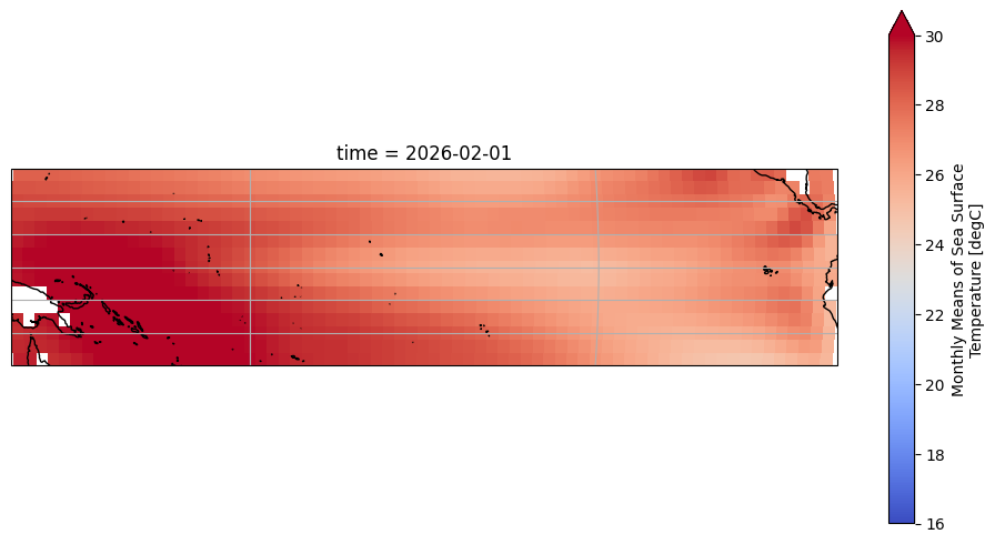
Let’s remove the monthly-mean seasonal cycle (aka the “climatology”) so that SST is expressed as anomalies around this cycle, as is the norm:

gb = ersstv5_tp.sst.groupby('time.month')
ersstv5_tpa = gb - gb.mean(dim='time')

Now extract the NINO3.4 index (a weighted average is involved, though it matters little so close to the equator because the weights are very close to unity):

nino34_anom = ersstv5_tpa.sel(lat=slice(5, -5), lon=slice(190, 240))
weights = np.cos(np.deg2rad(nino34_anom.lat))
nino34 = nino34_anom.weighted(weights).mean(dim=['lat', 'lon'])
nino34.plot()

[<matplotlib.lines.Line2D at 0x1791534d0>]

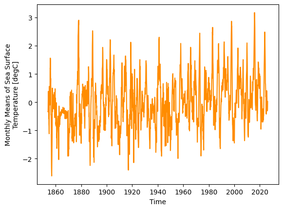
Now let’s leverage Pyleoclim’s integration with pandas to turn this into a Pyleoclim Series object. For this, we also leverage the fact that Xarray is pandas-based.

metadata = {
        'time_unit': 'years CE',
        'time_name': 'Time',
        'value_name': 'NINO3.4',
        'label': 'ERSST5 NINO3.4 index',
        'archiveType': 'Instrumental',
        'importedFrom': 'NOAA/NCEI',
    }

NINO34 = pyleo.Series.from_pandas(nino34.to_pandas(),metadata)
NINO34.plot()

(<Figure size 1000x400 with 1 Axes>,
 <Axes: xlabel='Time [years CE]', ylabel='NINO3.4'>)

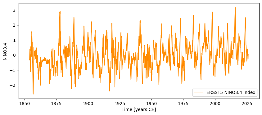
Notice how easy that was! One line of code is all it took to export the nino34 Xarray DataArray object as a pandas Series, and import it as a Pyleoclim Series (which is nothing more than a pandas Series with a little extra metadata to make life easier). Now we can deploy our correlation arsenal again, this time throwing in the T-test modified for the effects of serial correlation (ttest):

for method in ['built-in','ttest','ar1sim','phaseran']:
    corr_n = srca.correlation(NINO34,method=method)
    print(corr_n)

  statistic    critical value  p-value    signif. (α: 0.05)
-----------  ----------------  ---------  -------------------
  -0.453015               nan  < 1e-68    True

  statistic    critical value  p-value    signif. (α: 0.05)
-----------  ----------------  ---------  -------------------
  -0.453015           -0.1198  < 1e-3     True

Evaluating association on surrogate pairs: 100%|██████████| 1000/1000 [00:00<00:00, 1360.17it/s]

  statistic    critical value  p-value    signif. (α: 0.05)
-----------  ----------------  ---------  -------------------
  -0.453015         -0.143438  < 1e-6     True

Evaluating association on surrogate pairs: 100%|██████████| 1000/1000 [00:01<00:00, 967.01it/s]

  statistic    critical value  p-value    signif. (α: 0.05)
-----------  ----------------  ---------  -------------------
  -0.453015         -0.123136  < 1e-6     True

In this case, we see a correlation similar to what was observed between the Hulu and GISP2 records, but it appears highly significant no matter what test is used. The difference between the first two tests is instructive: we see how without accounting for serial correlation the p-value is a preposterous “<1e-68”, meaning basically impossible. Once serial correlation is accounted for (admittedly crudely), we get a p-value near \(10^{-3}\), which is quite a bit more conservative than those estimated with the Monte Carlo simulations (ar1sim,phaseran) near \(10^{-6}\). Notably, the critical value of the statistic is comparable for all methods that calculate it.

We now wish to carry out a similar analysis over the SST grid, so we write a simple loop. For computational convenience, we restrict ourselves to the T-test, which requires no Monte Carlo simulations. Notice how we use the same pandas trick as before as a cross-walk between xarray and Pyleoclim.

nlon = ersstv5_tpa.lon.size
nlat = ersstv5_tpa.lat.size
metadata = {
        'time_unit': 'years CE',
        'time_name': 'Time',
        'value_name': 'SST',
        'label': 'ERSST5 local SST',
        'archiveType': 'Instrumental',
        'importedFrom': 'NOAA/NCEI',
    }
series_list = []
for ji in range(nlon):
    metadata['lon'] = ersstv5_tpa.lon.values[ji]
    for jj in range(nlat):
        local_sst = ersstv5_tpa.isel(lon=ji,lat=jj)
        # check for land points
        if ~np.isnan(local_sst.values.mean()):
            metadata['lat'] = ersstv5_tpa.lat.values[jj]
            series = pyleo.GeoSeries.from_pandas(local_sst.to_pandas(),metadata)
            series_list.append(series)
            
print(len(series_list))        
sst_ms = pyleo.MultipleGeoSeries(series_list) 

1051

There over 1000 series in this collection, but the syntax is the same: we simply apply the correlation() method, and plot the result as we did for the Hulu and GISP2 ensemble correlation above:

corr_f = sst_ms.correlation(srca,method='ttest')
corr_f.plot()

Looping over 1051 Series in collection

100%|██████████| 1051/1051 [09:14<00:00,  1.90it/s]

(<Figure size 400x400 with 1 Axes>, <Axes: xlabel='$r$', ylabel='Count'>)

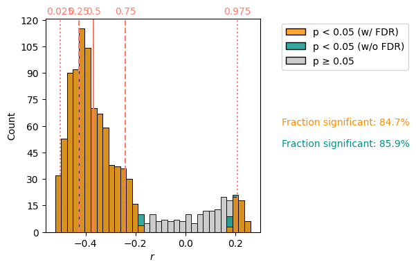
We see a bimodal distribution, with correlations close to 0 rejected as insignificant. In this case, the False Discovery Rate correction is very small, only changing the number of gridpoints significantly correlated to the Palmyra Sr/Ca record from 84.9% to 85.9%.

Takeaways

• pyleoclim allows to easily compute correlations between series with different time axes (including different resolutions).

• pyleoclim assesses significance with 3 different methods that are meant to guard against the deleterious effects of persistence, thereby lowering the risk of spurious correlations and p-hacking.

• pyleoclim allows to compute correlations between a series and a collection of series, e.g. coming from a gridded field, addressing the Multiple Hypothesis Problem with the False Discovery Rate.

• pyleoclim allows to compute correlations between, and within, MultipleSeries and EnsembleSeries object, using those same tools.

Acknowledgments

Project Pythia for this notebook on xarray manipulations

%watermark -n -u -v -iv -w

Last updated: Wed Jan 08 2025

Python implementation: CPython
Python version       : 3.11.9
IPython version      : 8.25.0

cartopy   : 0.23.0
xarray    : 2023.6.0
numpy     : 1.26.4
pyleoclim : 1.1.0b0
matplotlib: 3.8.4

Watermark: 2.4.3