
Spectral Analysis with Pyleoclim#
Preamble#
Goals#
Understand the various methods for spectral analysis accessible through Pyleoclim
Understand the effect of pre-processing on spectral analysis
Determine significance of spectral power
Reading time: 15 minutes
Keywords#
Spectral Analysis
Pre-requisites#
Pre-processing method available through Pyleoclim. An understanding of spectral analysis is a must.
Relevant Packages#
scikit-learn
Data Description#
This tutorial makes use of the following dataset, stored in CSV format:
Lisiecki, L. E., and Raymo, M. E. (2005), A Pliocene-Pleistocene stack of 57 globally distributed benthic δ18O records, Paleoceanography, 20, PA1003, doi:10.1029/2004PA001071.
Demonstration#
Let’s import the necessary packages:
%load_ext watermark

import pyleoclim as pyleo
import pandas as pd
import numpy as np
import matplotlib.pyplot as plt
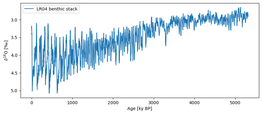
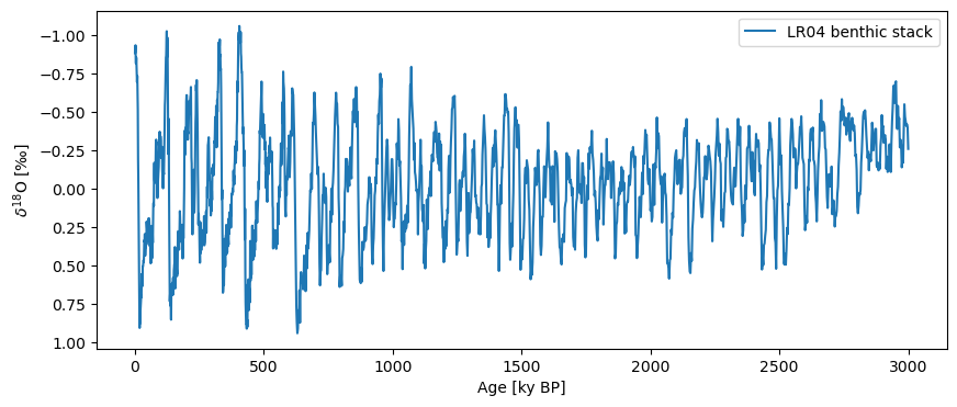
Let’s first import data and plot it so that up means “warm”:
lr04 = pyleo.utils.load_dataset('LR04')
fig, ax = lr04.plot(invert_yaxis=True)
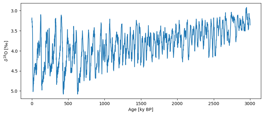
Let’s work with the first 3 million years (3000 kyr) of the record for illustrative purposes:
lr04_s = lr04.slice([0,3000])
fig,ax = lr04_s.plot(legend=False, invert_yaxis=True)
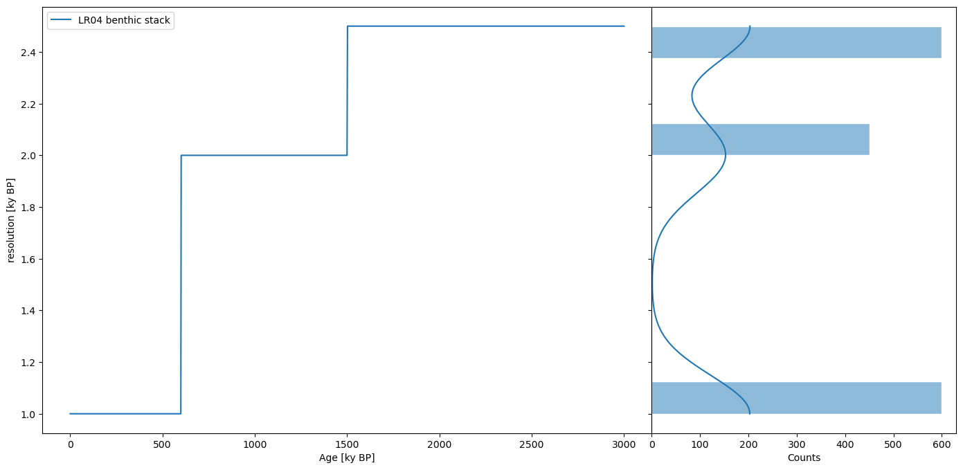
One important aspect of this dataset is that the resolution (spacing between observations) is variable, with 3 regimes:
lr04res = lr04_s.resolution()
lr04res.dashboard()
(<Figure size 1100x800 with 2 Axes>,
 {'res': <Axes: xlabel='Age [ky BP]', ylabel='resolution [ky BP]'>,
  'res_hist': <Axes: xlabel='Counts'>})
This requires caution, as the vast majority of spectral methods make the implicit assumption of uniform time spacing. In the following, we will illustrate strategies for how to deal with this difficulty.
Spectral methods#
Pyleoclim enables five spectral analysis methods:
Basic Periodogram, which uses a Fourier transform. The method has various windowing available to reduce variance.
Welch’s periodogram, a variant of the basic periodogram, which uses Welch’s method of overlapping segments. The periodogram of the full timeseries is the average of the segment periodograms.
Multi-taper method (MTM), which attempts to reduce the variance of spectral estimates by using a small set of tapers rather than the unique data taper or spectral window
Lomb-Scargle periodogram, an inverse approach designed for unevenly-spaced datasets. Several windows are available and Welch’s segmentation can also be used with this method.
Weighted wavelet Z-transform, a wavelet-based method also made for unevenly-spaced datasets.
All of these methods are available through Series.spectral by changing the method argument. Let’s have a look at the various methods. Since the first three methods require evenly-spaced data, we will be using a simple linear interpolation. The effect of pre-processing on the periodogram is discussed further in this notebook.
PSD_p = lr04_s.standardize().interp().spectral(method='periodogram')
fig, ax = PSD_p.plot(label = 'Periodogram')
lr04_s.standardize().interp().spectral(method='welch').plot(ax=ax,label='Welch')
lr04_s.standardize().interp().spectral(method='mtm').plot(ax=ax,label='MTM')
lr04_s.standardize().spectral(method='lomb_scargle').plot(ax=ax,label='Lomb Scargle')
lr04_s.standardize().spectral(method='wwz').plot(ax=ax,label='WWZ',lgd_kwargs={'bbox_to_anchor':(1.05, 1)})
OMP: Info #276: omp_set_nested routine deprecated, please use omp_set_max_active_levels instead.
<Axes: xlabel='Period [ky]', ylabel='PSD'>

These methods return similar answers, with peaks in the orbital bands at around ~23kyr, 40kyr, and (except for the Periodogram and Welch methods) 100kyr. This is not surprising given that the benthic stack is orbitally tuned. We would expect these periodicities to show up. The fact that the Periodogram and Welch methods miss the 100-kyr cycle is interesting.
But let’s have a look at the various arguments for the functions and let’s run down some of the important ones. In Pyleoclim, each of the method parameters should be passed through the argument settings, which takes a dictionary of possible key/value that corresponds to the argument of the underlying function. Look at the See also section in the documentation. From there, you can have a look at the parameters for the specific methods.
Periodogram#
The most important parameter here is window which corresponds to the type of window to be used to reduce the variance. If you are interested in seeing the impact of these windows on a spectrum, look at this documentation. The detrend, gaussianize, and standardize parameters correspond to pre-processing steps that can either be passed directly to the function or with method cascading. I prefer using the dedicated functions rather than the parameters as it makes it easier to follow the order in which these operations occurred.
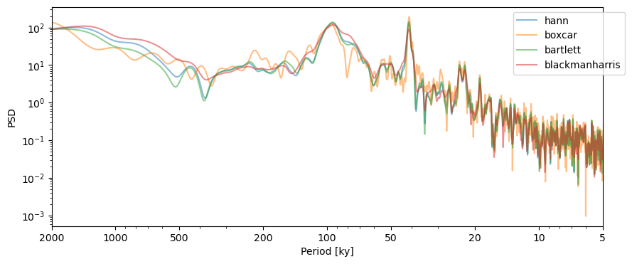
For the purpose of this tutorial, let’s consider the following windows: boxcar, bartlett, and blackmanharris (note that the default window is hann):
PSD_boxcar = lr04_s.standardize().interp().spectral(method='periodogram', settings={'window':'boxcar'})
fig,ax = PSD_boxcar.plot(label = 'boxcar')
lr04_s.standardize().interp().spectral(method='periodogram', settings={'window':'bartlett'}).plot(ax=ax,label='bartlett')
lr04_s.standardize().interp().spectral(method='periodogram', settings={'window':'blackmanharris'}).plot(ax=ax,label='blackmanharris')
<Axes: xlabel='Period [ky]', ylabel='PSD'>
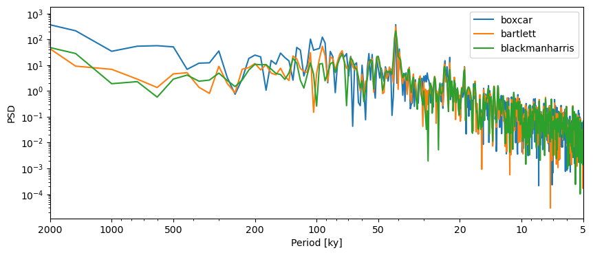
The periodograms look very similar, except for the 100-kyr band, which could be interpreted as present (albeit maybe not significant) when using a boxcar window. This example highlights the danger of over-interpreting peaks in spectral analysis.
Welch#
Welch’s method divides the series into segments to obtain a more stable estimate of the periodogram. Besides window, the two relevant parameters are nperseg and noverlap, which correspond to the number of points and fraction of overlap (in %), respectively. The default will give you three segments with 50% overlap. Let’s look at 4,5,6 segments with 50% overlap:
PSD_welch = lr04_s.standardize().interp().spectral(method='welch')
fig,ax = PSD_welch.plot(label='3 segments, 50% overlap')
lr04_s.standardize().interp().spectral(method='welch', settings = {'nperseg':len(lr04_s.value)/3}).plot(ax=ax,label='4 segments, 50% overlap')
lr04_s.standardize().interp().spectral(method='welch', settings = {'nperseg':len(lr04_s.value)/3}).plot(ax=ax,label='5 segments, 50% overlap')
<Axes: xlabel='Period [ky]', ylabel='PSD'>
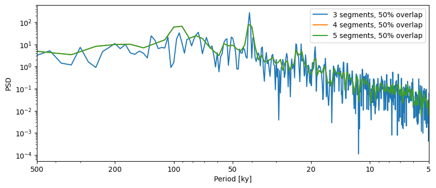
This, again, cautions against over interpreting the 100-kyr peak in the data.
MTM#
The most important parameter for MTM is the time-bandwidth product NW, which controls the amount of leakage out of a given spectral line (see. Ghil et al, 2002). This parameter is usually set between 2 and 4 (which is the default for Pyleoclim) in increments of 1/2. 4 is the most conservative choice advocated by MTM’s originator (D. Thomson), though the code allows you to go higher (and therefore, smoother) if you think that is warranted:
PSD_nw4 = lr04_s.standardize().interp().spectral(method='mtm')
fig,ax = PSD_nw4.plot(label= 'NW:4.0')
for item in np.flip(np.arange(2,4,0.5)):
    lr04_s.standardize().interp().spectral(method='mtm', settings={'NW':item}).plot(ax=ax, label = 'NW:'+str(item), alpha=0.5, lgd_kwargs={'bbox_to_anchor':(1.05, 1)})
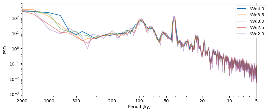
Let’s have a look at the effect of NW on the spectrum. As NW decreases, the peaks become sharper. This is particularly apparent in the 2000 kyr band (which corresponds to the trend in data; as we will see shortly), whereas the peak corresponding to \(NW=4\) is much broader. The trade-off (there always is one in spectral analysis) is that the variance is higher for smaller values of NW (it cannot be seen on this plot, but it means that there is more uncertainty as to the height of a narrow peak than a diffuse one).
Lomb-Scargle#
The Lomb-Scargle periodogram is meant to work with unevenly-spaced timeseries. The parameters of importance here are:
The frequency vector, which can either be user-specified or calculated using different methods (
'log','lomb_scargle','welch', 'scale', 'nfft'), which determines at which points in the frequency domain the periodogram should be computed. This a trade-off: if using too many points, some peaks might be spurious. Not enough, and you can miss some significant periodicities. There is also a computational trade-off here: the more points, the longer it takes for the code to run.n50: which determines the number of overlapping segments with 50% overlap using the Welch method
window, as we have seen for the periodogram.
Note: The Series.spectral method overwrites the default ‘lomb-scargle’ method for this function and uses ‘log’ as its frequency method.
Let’s take a look at the effect of these parameters one by one. Also notice that the data need no interpolation with this method.
freq (Frequency vector)#
freq = np.arange(1/2000,1/5,1/10) # a user defined one to get started. This one should be passed through settings

PSD_ls = lr04_s.standardize().spectral(method='lomb_scargle',freq=freq)
fig,ax = PSD_ls.plot(label = 'User-defined frequency',alpha=0.5)

freq_methods = ['nfft','log','lomb_scargle','welch', 'scale']
for freq_method in freq_methods:
    lr04_s.standardize().spectral(method='lomb_scargle',
                                  freq=freq_method).plot(ax=ax,label=freq_method,alpha=0.5, lgd_kwargs={'bbox_to_anchor':(1.05, 1)})
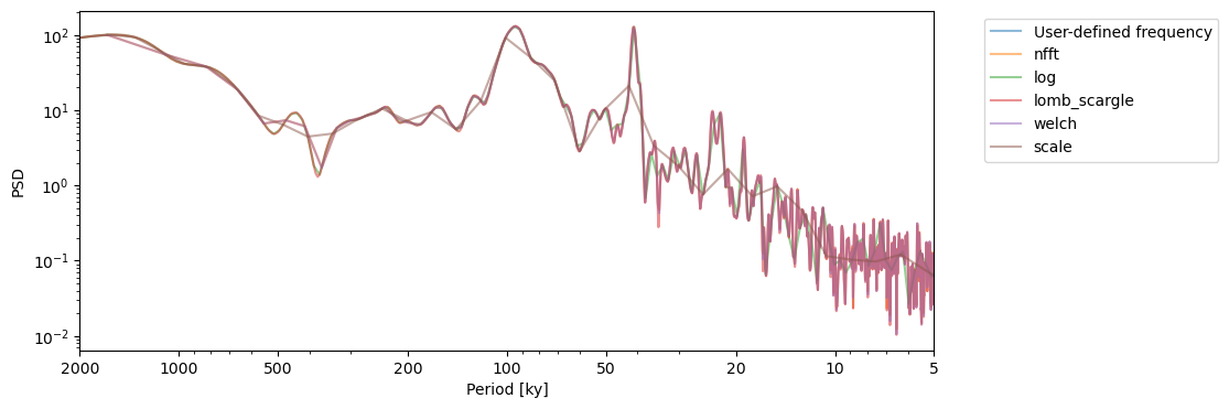
Note how the 40-kyr peak is poorly defined using the frequency vector from the scale method.
n50#
Let’s look at the effect of segmentation. The default is to use 3 segments with 50% overlap.
PSD_ls = lr04_s.standardize().spectral(method='lomb_scargle', settings={'n50':1})
fig,ax = PSD_ls.plot(label = 'n50=1',alpha=0.5)

n50s = np.arange(2,6,1)
for item in n50s:
    lr04_s.standardize().spectral(method='lomb_scargle', settings={'n50':item}).plot(ax=ax,label='n50='+str(item),alpha=0.5, lgd_kwargs={'bbox_to_anchor':(1.05, 1)})
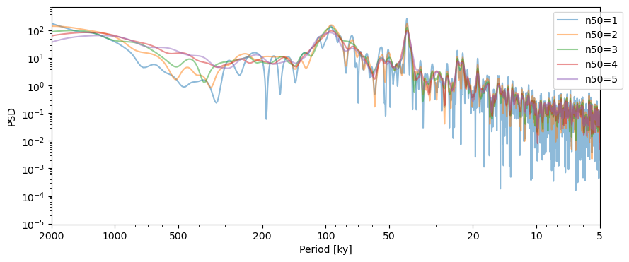
By design, Welch’s method shows less variance (smoother spectra) with a greater number of segments. The trade-off here is since the spectrum is estimated on a smaller portion of the timeseries, low-frequency cycles (if any) can be lost in the segments. In order to look at low-frequency cyclicities that may only repeat 3-4 times, set n50 as low as possible.
window#
Let’s examine the behavior with the windows we selected above: boxcar, bartlett, and blackmanharris. Note that Lomb-Scargle is the default method in Pyleoclim, so we will not set that argument in the example.
window =  ['boxcar', 'bartlett', 'blackmanharris']

PSD_ls = lr04_s.standardize().spectral()
fig,ax = PSD_ls.plot(label = 'hann',alpha=0.5)

for item in window:
    lr04_s.standardize().spectral(settings={'window':item}).plot(ax=ax,alpha=0.5,label = item, lgd_kwargs={'bbox_to_anchor':(1.05, 1)})
The choice of window is not as critical as with the basic Fourier periodogram.
WWZ#
Spectral density can be computed from the weighted wavelet Z transform wavelet method in one of two ways:
use the method through the
spectral()method of theSeriesclass, as above (most users).If you had previously calculated a scalogram, you can then obtain a PSD from it.
However, the results will not be interchangeable. Let us see why:
Method 1: Use the Series.spectral method#
psd_wwz_d = lr04_s.standardize().spectral(method='wwz')
Method 2: Compute PSD through a scalogram#
Step 1: use the wavelet function to calculate the scalogram. Step 2: pass the computed scalogram to the scalogram parameter in the spectral function:
scal = lr04_s.standardize().wavelet(method='wwz')
psd_wwz = lr04_s.standardize().spectral(method='wwz',scalogram=scal)
Now let’s plot them and compare:
fig,ax = psd_wwz.plot(label='Computed through wavelet function')
psd_wwz_d.plot(ax=ax, label='Computed through spectral function',
               lgd_kwargs={'bbox_to_anchor':(1.05, 1)})
<Axes: xlabel='Period [ky]', ylabel='PSD'>
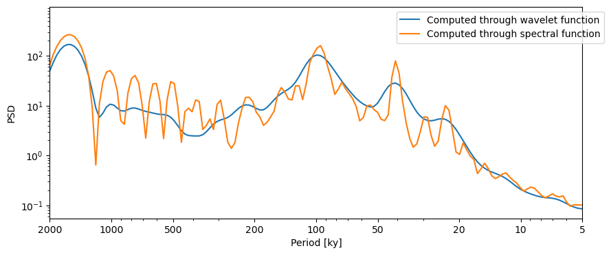
Big difference!!! So what’s happening here? Let’s have a look at the various implementations:
Both WWZ implementations use a parameter called c, the wavelet’s decay constant. This constant balances the time resolution and frequency resolution of the wavelet analysis. The smaller this constant is, the sharper the peaks. For spectral analysis, where the purpose is to find peaks over the entirely of the series, a small value for c is useful. In contrast, wavelet analysis relies on time-frequency localization, which requires a larger value of c, hence a smoother spectrum when averaged over time. If you look at the defaults for these two functions, c takes on different values for each of the cases.
So why did we enable the passing of scalograms if they’re not appropriate to use? The short answer is time. It may not have felt this way here, but the WWZ algorithm is considerably slower than the other spectral methods. When computing one periodogram, this is not an issue. However, for significance testing, this can be rather time-consuming. Therefore, passing the scalograms can be sufficient for preliminary data exploration.
Determining significance#
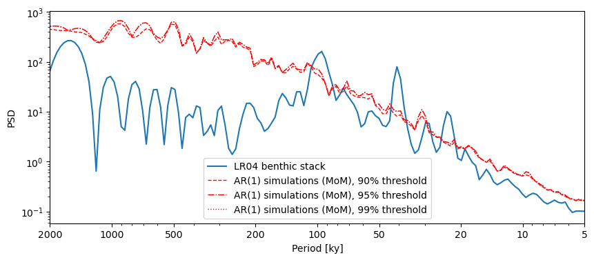
Great, we’ve found peaks. Now it’s time to determine whether said peaks are significant. That is: do they stand out compared to what one might expect to see in a random timeseries? By default, Pyleoclim tests against an AR(1) benchmark, simulating surrogates of the time series. Let’s use this on the Lomb-Scargle method and test against 90%, 95%, and 99% significance level through the PSD.signif_test. The qs parameter is adjusted for the desired significance levels.
psd_ls = lr04_s.standardize().spectral()
psd_ls.signif_test(qs=[0.90,0.95,0.99]).plot()
Using serial execution for this method on a Mac platform
Performing spectral analysis on individual series: 100%|██████████| 200/200 [01:49<00:00, 1.82it/s]
(<Figure size 1000x400 with 1 Axes>,
 <Axes: xlabel='Period [ky]', ylabel='PSD'>)
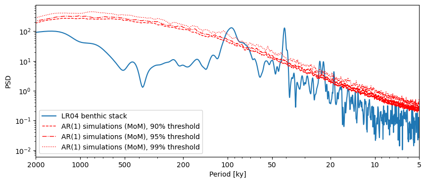
According to the significance testing, the peaks corresponding to orbital cylicities are significant in the data. I would still interpret the 100-kyr peak with caution given that other methods cannot identify it.
What other parameters are available? One is number which sets the number of surrogates to generate. Notice how the 99% threshold is not smooth. This is due to the fact that, by default, the method uses only 200 surrogates, so the 99% quantile in only \(n=2\). Let’s increase that number to 1000:
psd1000 = psd_ls.signif_test(number=1000,
                   qs=[0.90,0.95,0.99])
psd1000.plot()
Using serial execution for this method on a Mac platform
Performing spectral analysis on individual series: 100%|██████████| 1000/1000 [09:15<00:00, 1.80it/s]
(<Figure size 1000x400 with 1 Axes>,
 <Axes: xlabel='Period [ky]', ylabel='PSD'>)
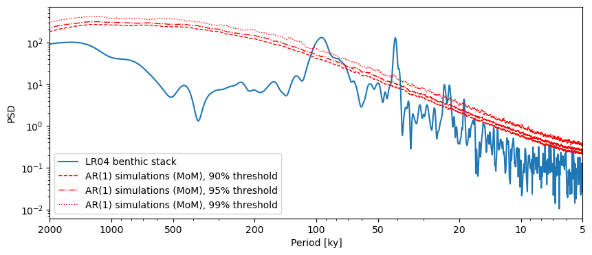
This took about 5 times longer (about 3 and a half minutes on my laptop). That is acceptable considering how much smoother the threshold look. And what is 3.5min compared to months of a paper lingering in peer-review limbo?
You might ask, if it’s only 3.5, why is the default 200? Because the WWZ method takes significantly more time. Let’s try 10 surrogates to give you an idea:
lr04_s.standardize().spectral(method='wwz').signif_test(number=10,
                                                        qs=[0.90,0.95,0.99]).plot()
Performing spectral analysis on individual series:   0%|          | 0/10 [00:00<?, ?it/s]OMP: Info #276: omp_set_nested routine deprecated, please use omp_set_max_active_levels instead.
OMP: Info #276: omp_set_nested routine deprecated, please use omp_set_max_active_levels instead.
OMP: Info #276: omp_set_nested routine deprecated, please use omp_set_max_active_levels instead.
OMP: Info #276: omp_set_nested routine deprecated, please use omp_set_max_active_levels instead.
OMP: Info #276: omp_set_nested routine deprecated, please use omp_set_max_active_levels instead.
OMP: Info #276: omp_set_nested routine deprecated, please use omp_set_max_active_levels instead.
OMP: Info #276: omp_set_nested routine deprecated, please use omp_set_max_active_levels instead.
OMP: Info #276: omp_set_nested routine deprecated, please use omp_set_max_active_levels instead.
OMP: Info #276: omp_set_nested routine deprecated, please use omp_set_max_active_levels instead.
OMP: Info #276: omp_set_nested routine deprecated, please use omp_set_max_active_levels instead.
Performing spectral analysis on individual series: 100%|██████████| 10/10 [00:10<00:00,  1.02s/it]
(<Figure size 1000x400 with 1 Axes>,
 <Axes: xlabel='Period [ky]', ylabel='PSD'>)
Running the analysis over 10 surrogates took about 1 minute. Therefore, 200 would take about 20 minutes and 1000 would take 1hr 40min to run. To be sure, 10 surrogates are not enough to make a determination about significance (as attested by the very jagged red lines), but 20 min is a good compromise between computation time and statistical accuracy.
Assessing scaling behavior#
Another important element of spectral analysis is the estimation of scaling behavior, which typically inform about rates of tranfer between different scales of variation. Scaling is quantified by an exponent \(\beta\) such that the PSD \(S(f)\) obeys a power law: $\( S(f) \propto f^{-\beta}\)$
Estimating scaling exponents#
Pyleoclim makes it easy to estimate scaling exponents (and their uncertaintiy) via the function beta_est():
psd_ls.beta_est().plot()
(<Figure size 1000x400 with 1 Axes>,
 <Axes: xlabel='Period [ky]', ylabel='PSD'>)
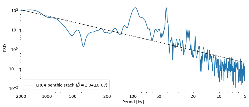
The exponent itself is stored in a dictionary called beta_est_res :
psd_ls.beta_est().beta_est_res['beta']
np.float64(1.0416492485108377)
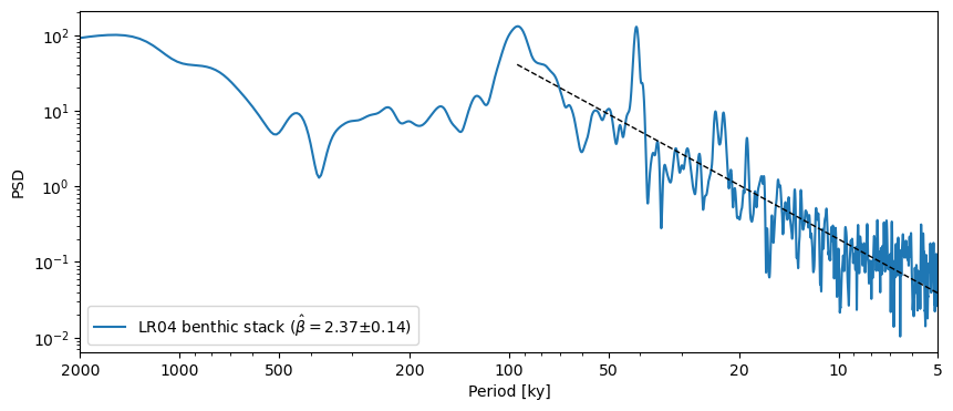
By default, the exponent is estimated over the entire spectrum. If you need to refine the range over which the exponent is estimated, you may specify a minimum and maximum frequency:
psd_ls.beta_est(fmin=1/100, fmax=1/5).plot()
(<Figure size 1000x400 with 1 Axes>,
 <Axes: xlabel='Period [ky]', ylabel='PSD'>)
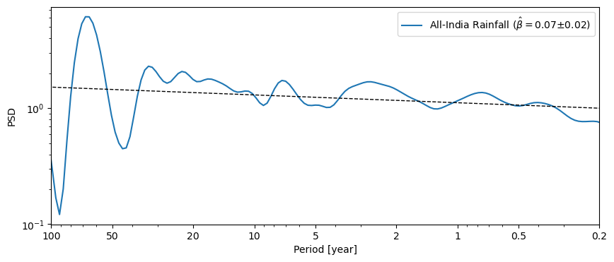
Effect of aliasing#
Aliasing is a common scourge of spectral analysis, and is particularly injurious to records that exhibit scaling behavior. The problem does not seem to affect LR04, so let us look at AIR instead:
ts = pyleo.utils.load_dataset('AIR')
psd_alias = ts.spectral(method='cwt')
psd_alias.beta_est().plot()
(<Figure size 1000x400 with 1 Axes>,
 <Axes: xlabel='Period [year]', ylabel='PSD'>)
The anti-alias filter proposed by Kirchner (2005) is implemented in anti_alias():
psd_anti = psd_alias.anti_alias().beta_est().plot()
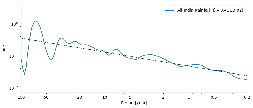
We see that this did increase the slope quite a bit. However, be careful in applying this adjustment that the signal truly was generated by a process with a spectrum that scales like \(f^{-\beta}\). If you don’t have strong suspicions/evidence that this is the case, best not apply this correction, lest the remedy be worse than the ill.
Effect of pre-processing on spectral analysis#
Often times, the time series needs the following pre-processing steps:
standardization: this is a must for most of our techniques
even sampling: needed for methods that do not take unevenly-spaced data natively (MTM, Periodogram, and Welch). Pyleoclim offers several regridding options, whose impacts on spectral analysis are explored here
detrending
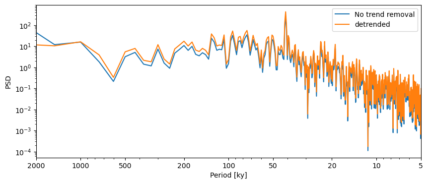
Effect of detrending#
The LR04 curve has a trend over the past 3 million years, which corresponds to increased ice volume from long-term cooling of the Earth and growth of polar ice caps, which enrich the oceans in the heavy oxygen isotope. Let’s remove the trend:
ts = lr04_s.detrend().plot(invert_yaxis=True)
Let’s compare the two periodograms using the Lomb-Scargle method:
fig,ax = lr04_s.standardize().spectral().plot(label = 'No trend removal')
lr04_s.detrend().standardize().spectral().plot(ax=ax,label='detrended')
<Axes: xlabel='Period [ky]', ylabel='PSD'>
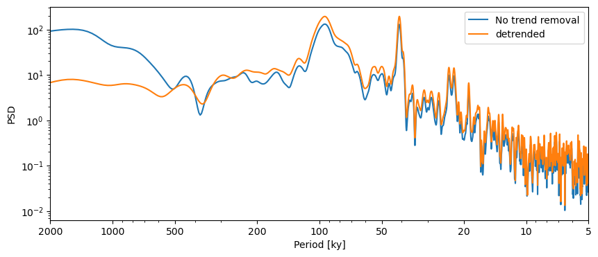
In this case, the detrending doens’t seem to matter much in the interpretation of our results.
fig,ax = lr04_s.interp().standardize().spectral(method='periodogram').plot(label = 'No trend removal')
lr04_s.detrend().interp().standardize().spectral(method='periodogram').plot(ax=ax,label='detrended')
<Axes: xlabel='Period [ky]', ylabel='PSD'>
For more details on detrending, see the tutorial on filtering and detrending.
Effect of regridding#
For the spectral methods requiring evenly-spaced data (such as MTM), imputation is needed. Let’s run through various methods:
linear interpolation
spline interpolation
binning
Gaussian kernel
method = ['linear interpolation', 'spline interpolation', 'binning', 'Gaussian kernel']

fig, ax = plt.subplots(figsize=[10,4])

for item in method:
    if item == 'linear interpolation':
        lr04_s.detrend().interp().standardize().spectral(method='mtm').plot(ax=ax,label=item)
    elif item == 'spline interpolation':
        lr04_s.detrend().interp(method='cubic').standardize().spectral(method='mtm').plot(ax=ax,label=item)
    elif item == 'binning':
        lr04_s.detrend().bin().standardize().spectral(method='mtm').plot(ax=ax,label=item)
    elif item == 'Gaussian kernel':
        lr04_s.detrend().gkernel().standardize().spectral(method='mtm').plot(ax=ax,label=item)
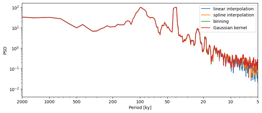
The type of imputation doesn’t matter for this application. However, we have used the default parameters for each of these techniques for the step size, which refers to the interpolation step. The default is the mean time increment, but it can be adjusted to taste. Let’s use the Resolution class, which we used earlier, to quickly obtain these parameters:
res_stats = lr04res.describe()
res_stats
{'nobs': np.int64(1650),
 'minmax': (np.float64(1.0), np.float64(2.5)),
 'mean': np.float64(1.8181818181818181),
 'variance': np.float64(0.42174320524835984),
 'skewness': np.float64(-0.30064837098248426),
 'kurtosis': np.float64(-1.6386966551326412),
 'median': np.float64(2.0)}
min_step, max_step = res_stats['minmax'] # minimum and maximum spacing between samples
fig,ax = lr04_s.detrend().interp().standardize().spectral(method='mtm').plot(label='mean resolution')
lr04_s.detrend().interp(step=min_step).standardize().spectral(method='mtm').plot(ax=ax, label='min resolution')
lr04_s.detrend().interp(step=max_step).standardize().spectral(method='mtm').plot(ax=ax, label='max resolution')
<Axes: xlabel='Period [ky]', ylabel='PSD'>
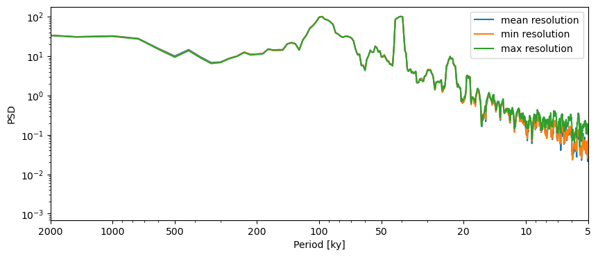
There are very marked differences in the 5-20ky range, but none beyond that.
Summary#
The 23ky and 41ky appear to be robust features of the LR04 benthic stack. As we saw earlier, the picture is less clear for the 100ky cycle, which appears clearly with some methods/parameter choices but not others. Our job is not to adjudicate this question, however. This is merely a tutorial. Your job is to leverage the versatility of Pyleoclim to make sure your results are not artifacts of arbitrary procedural choices.
%watermark -n -u -v -iv -w
Last updated: Thu, 12 Mar 2026

Python implementation: CPython
Python version       : 3.12.11
IPython version      : 9.6.0

matplotlib: 3.10.6
numpy     : 2.3.3
pandas    : 2.3.3
pyleoclim : 1.2.1b0

Watermark: 2.6.0