3.4 Comparing methods
This pre-processing allows us to better isolate oscillatory behavior. To see this, let’s look at the spectra of the original and detrended versions:
library(astrochron)

mtmOrig <- astrochron::mtm(dat = gmst,output = 1,verbose = F,genplot = F) %>%
  select(Frequency,Power) %>%
  mutate(data = "Original",
         period = (1/Frequency))


mtmSSA <- astrochron::mtm(dat = gmst_ssa_dtd,output = 1,verbose = F,genplot = F) %>%
  select(Frequency,Power) %>%
  mutate(data = "SSA-detrended",
         period = (1/Frequency))

library(scales)
reverselog_trans <- function(base = exp(1)) {
    trans <- function(x) -log(x, base)
    inv <- function(x) base^(-x)
    trans_new(paste0("reverselog-", format(base)), trans, inv,
              log_breaks(base = base),
              domain = c(1e-100, Inf))
}

bind_rows(mtmOrig,mtmSSA) %>%
  ggplot() +
  geom_line(aes(x = period,y = Power)) +
  scale_x_continuous(trans = reverselog_trans(10),breaks = c(100,50,20,10,5,2),limits = c(100,2)) +
  scale_y_log10() +
  facet_grid(data ~ .) +
  theme_light()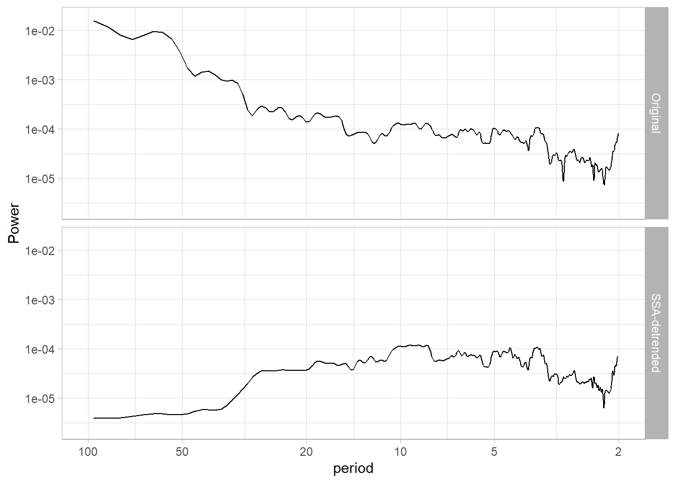
We see that detrending has removed much of the variability at scales longer than ~30y, allowing us to hone in on various peaks near 3.5, 6, 10, and 20 years. To see if those are significant, however, you would need to apply a significance test, which we would cover in another tutorial.