5.2 Data preview
First, let us inspect the distribution of values:
hist(df$`discharge (cf/s)`, main = "Distribution of Rio Grande Discharge", xlab = "Discharge (cf/s)")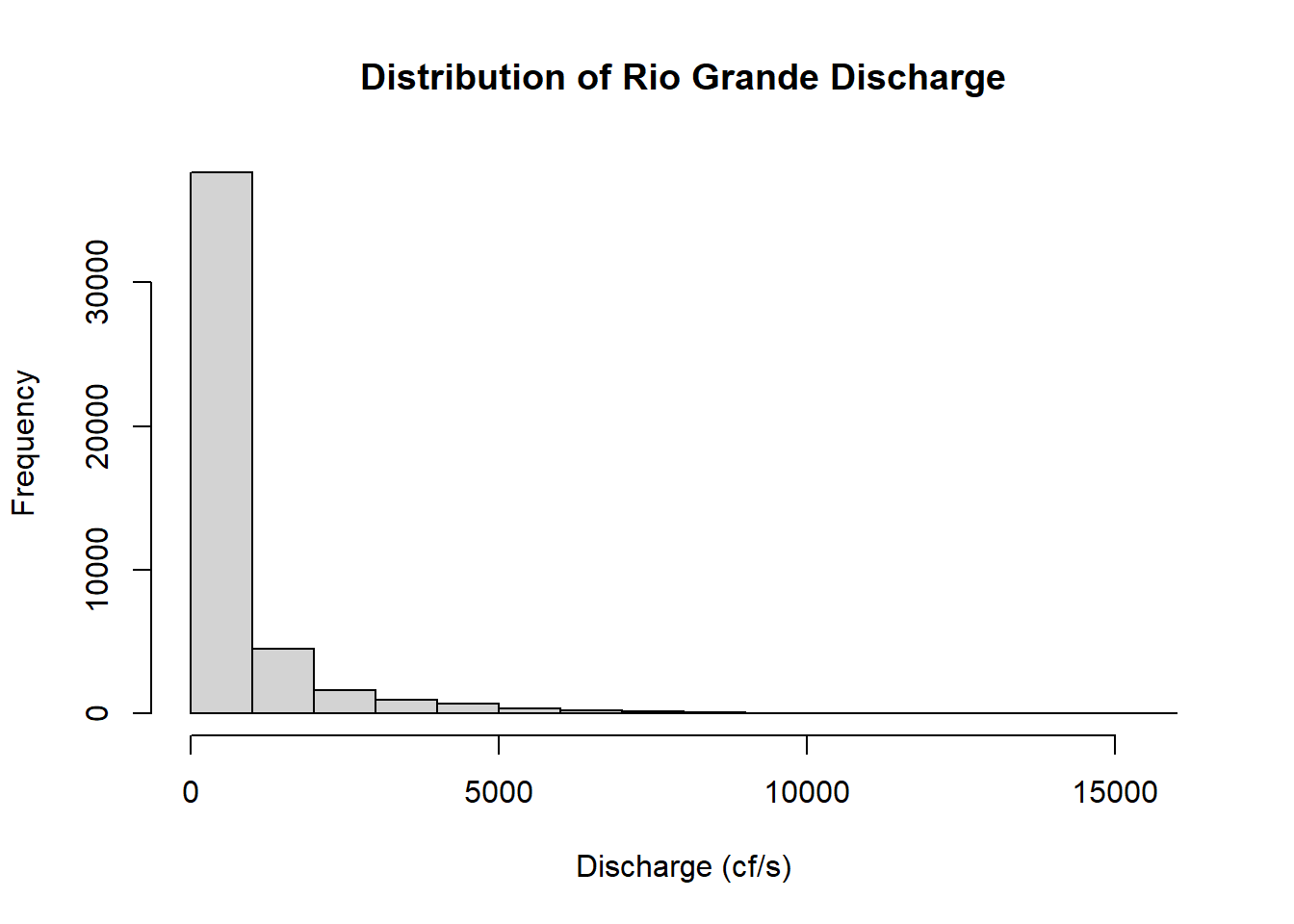
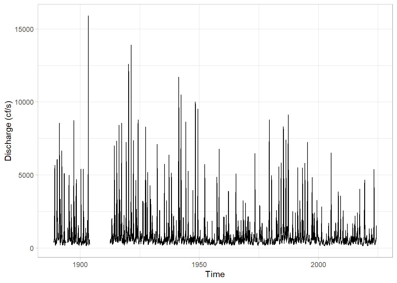
Like many other variables, streamflow is positively skewed: the distribution is asymmetric, with most values near zero and few instances of very high streamflow. Now let’s inspect the temporal behavior:
ggplot(df, aes(x = datetime, y = `discharge (cf/s)`)) +
  geom_line() +
  labs(x = "Time", y = "Discharge (cf/s)") +
  theme_light()