6.3 Sampling interval

First, take a look at the distribution of time increments. We’ll use the base function diff() to extract the sampling intervals.

deltaT <- data.frame("ID" = 1:(length(dDdf$AgeKy)-1),
                     "interval" = diff(dDdf$AgeKy))

ggplot(data = deltaT, mapping = aes(x=interval)) + 
  geom_histogram() +
  theme_light()

## `stat_bin()` using `bins = 30`. Pick better value with `binwidth`.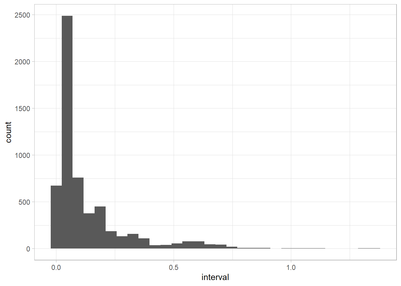

The data are not evenly spaced, which is a challenge because most timeseries analysis methods (particularly Fourier and wavelet analysis) make the implicit assumption that data are evenly spaced, so applying those tools to unevenly-spaced data will result in methods not behaving as they are supposed to. We therefore interpolate the data at 500y resolution to enable the much faster CWT algorithm of Torrence & Compo (1998) to run. We also standardize because the original data range is rather large, which could cause numerical issues.