3.3 Detrending |

3.3 Detrending

Now let’s move on to detrending. We’ll use the HadCRUT5 global mean surface temperature dataset.

gmst <- read_csv("https://github.com/LinkedEarth/Pyleoclim_util/raw/master/pyleoclim/data/HadCRUT.5.0.1.0.analysis.summary_series.global.annual.csv") %>% 
  select(time = Time,temp = `Anomaly (deg C)`)

ggplot(gmst, aes(x = time, y = temp)) +
  geom_line() +
  labs(x = 'Time [year C.E.]', y = 'GMST [°C]') +
  theme_light()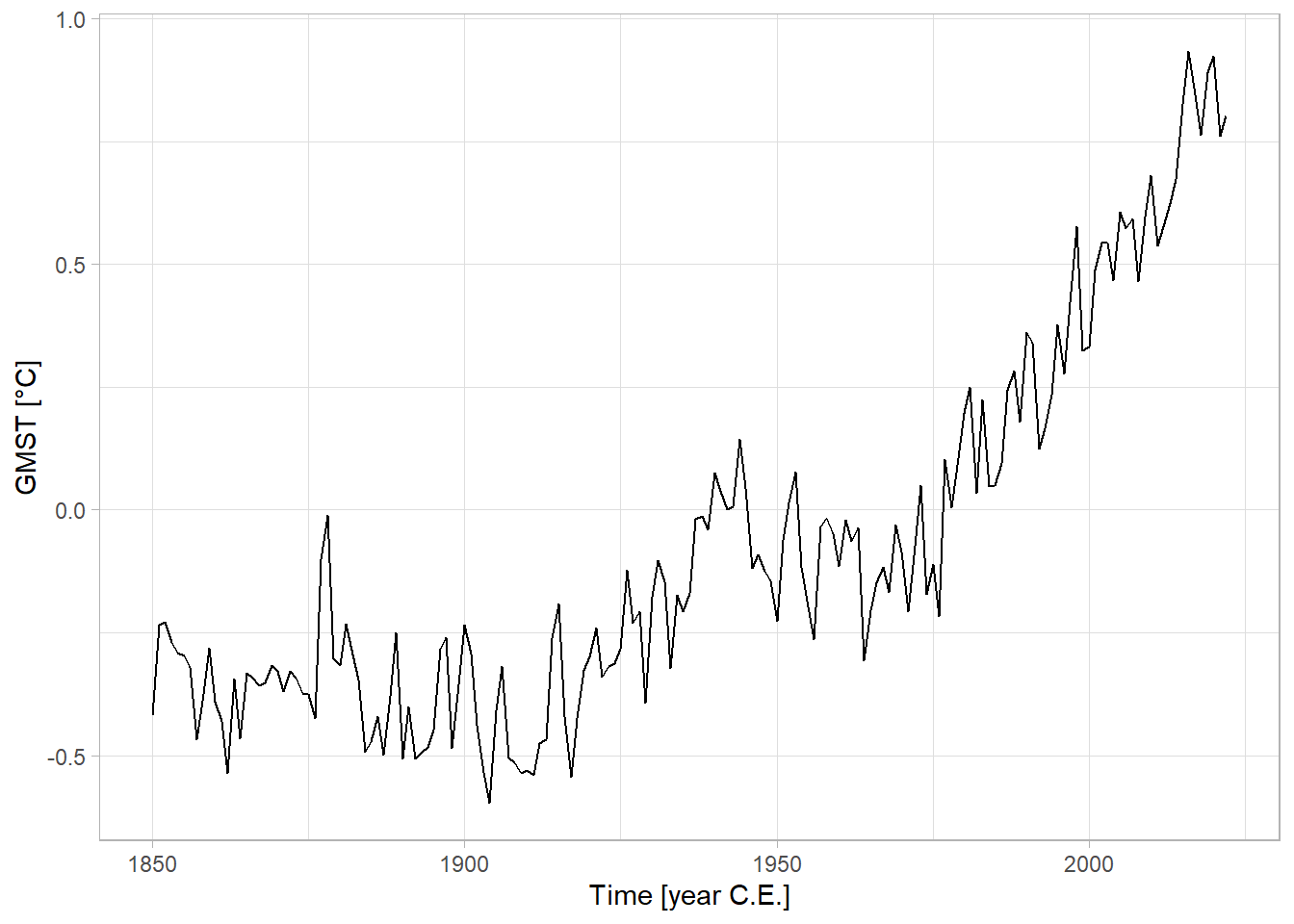

3.3.1 Detrending methods in R

Let’s apply 3 methods: linear detrending, Empirical Mode Decomposition (EMD), and Savitzky-Golay filter:

# Linear detrending
gmstLinear <- gmst
gmstLinear$detrended <- pracma::detrend(gmstLinear$temp)
gmstLinear$trend <- gmstLinear$temp - gmstLinear$detrended
gmstLinear$method <- "Linear"


# EMD using the EMD package
library(EMD)
emd_result <- emd(gmst$temp, boundary='symmetric', max.imf=4)

gmstEmd <- gmst
gmstEmd$detrended <- gmst$temp-emd_result$residue
gmstEmd$trend <- gmstEmd$temp - gmstEmd$detrended
gmstEmd$method <- "EMD"

# Savitzky-Golay filter
gmstSg <- gmst
gmstSg$trend <- signal::sgolayfilt(gmst$temp, p = 3, n = 51)
gmstSg$detrended <- gmst$temp - gmstSg$trend
gmstSg$method <- "Savitzky-Golay"

#prepare the data for plotting
gmstToPlot <- dplyr::bind_rows(gmstLinear,gmstEmd,gmstSg) %>% 
  tidyr::pivot_longer(cols = -c(time,method),values_to = "Temperature",names_to = "options") %>% 
  mutate(method = factor(method,levels = c("Linear","EMD","Savitzky-Golay")))

# Plot it!
ggplot(gmstToPlot) + 
  geom_line(aes(x = time, y = Temperature, color = options)) +
  facet_grid(method ~ .) +
  theme_light()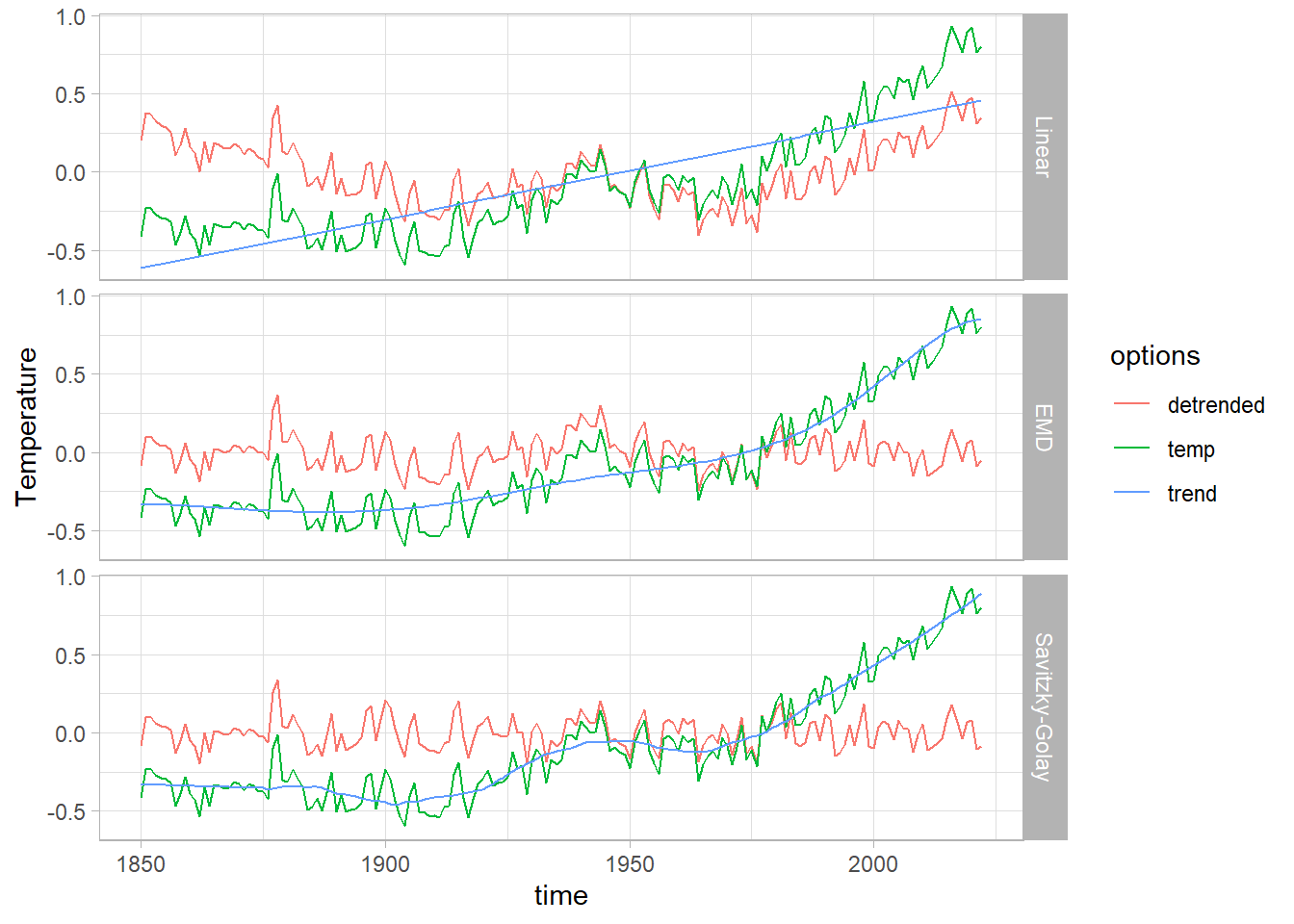

The linear trend here does a decent job at capturing first-order behavior. The EMD (approximated by SSA) and Savitzky-Golay methods also capture the nonlinear trend.

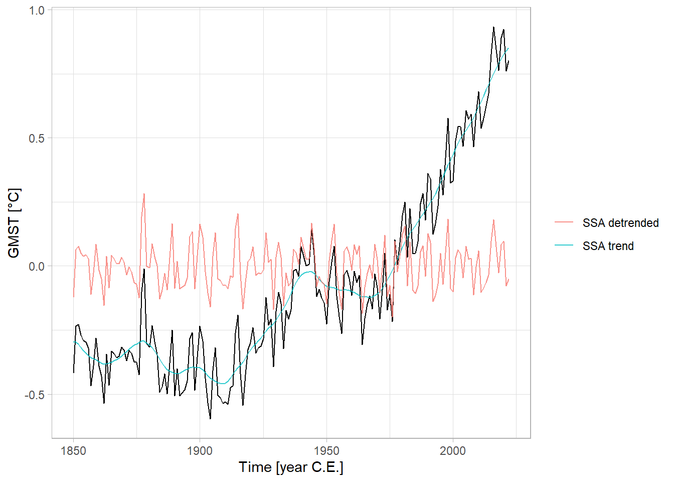
3.3.2 SSA detrending

Another option to isolate a non-linear trend is Singular Spectrum Analysis (SSA). If there is a prominent trend, it is often the first mode coming out of that analysis.

gmst_ssa <- ssa(gmst$temp, L = 10)
plot(gmst_ssa)

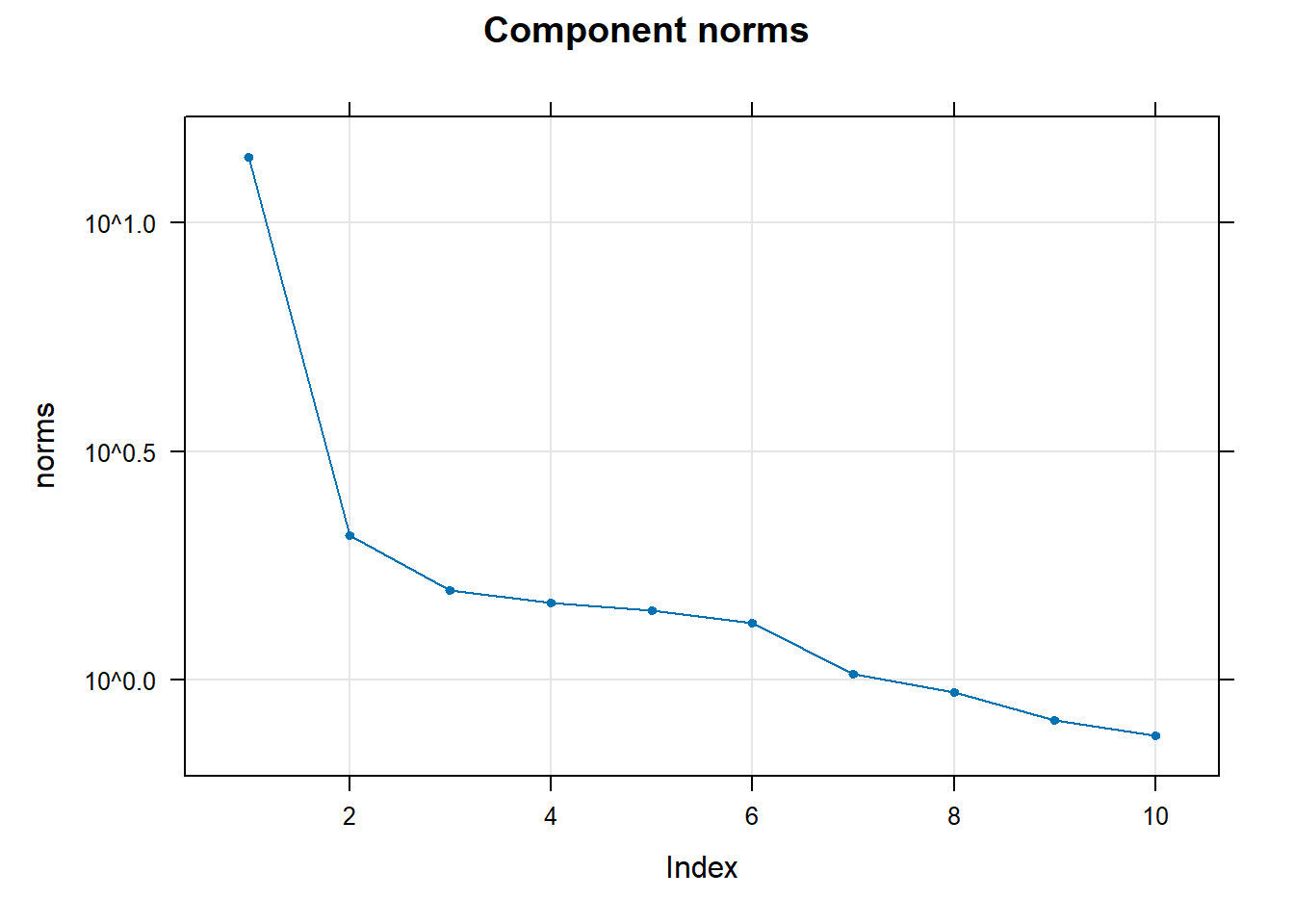
The first mode accounts for most fraction of the variance. Let’s compute this:

paste0(round(gmst_ssa$sigma[1] / sum(gmst_ssa$sigma),3) * 100,"%")

## [1] "55%"

Let’s use this mode as the trend:

ssa_trend <- reconstruct(gmst_ssa, groups = list(trend = 1))
gmst_ssa_dtd <- data.frame(time = gmst$time, temp = gmst$temp - ssa_trend$trend)

ggplot(gmst, aes(x = time, y = temp)) +
  geom_line() +
  geom_line(aes(y = ssa_trend$trend, color = "SSA trend"), alpha = 0.8) +
  geom_line(aes(y = gmst_ssa_dtd$temp, color = "SSA detrended"), alpha = 0.8) +
  labs(x = 'Time [year C.E.]', y = 'GMST [°C]', color = '') +
  theme_light()