3.2 Filtering
3.2.1 Data spacing
The goal of filtering is to enhance part of a signal, or suppress one or more parts. We’ll use R’s signal package, which provides a variety of filters.
First, let’s check if the data is evenly spaced:
diff_time <- data.frame(resolution= diff(df$time),
                        time =rowMeans(cbind(df$time[-1],df$time[-length(df$time)])))

#make a histogram of the options
ggplot(diff_time) +
  geom_line(aes(x = time,y = resolution)) +
  labs(x = 'time [s]', y = 'time difference [s]', title = 'Resolution') +
  theme_light()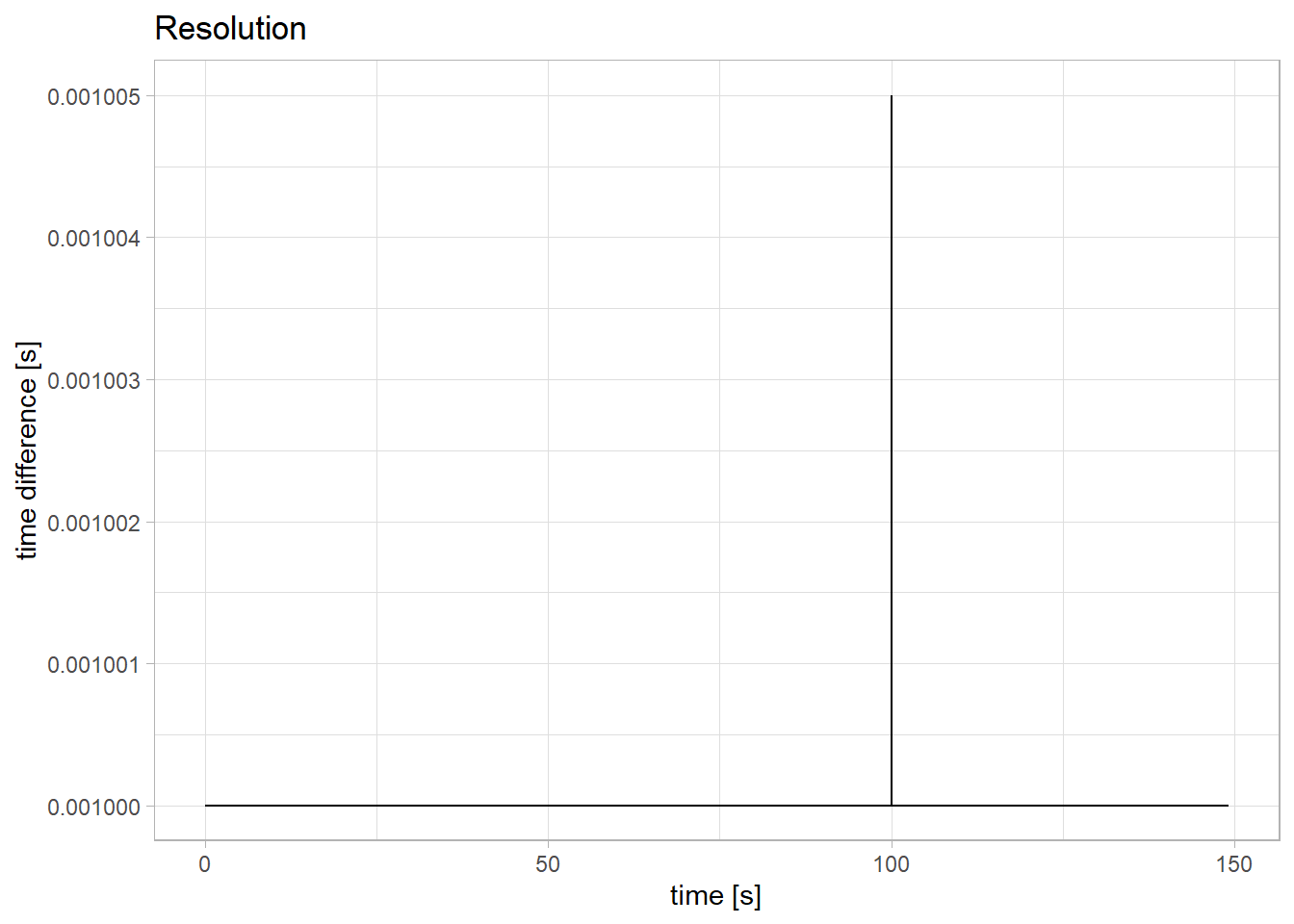
It appears that the resolution jumps at around the 100th second. Let’s interpolate to get an even resolution of 1ms:
ts <- zoo(df$ground_motion, df$time)
ts_interp <- na.approx(ts, xout = seq(min(df$time), max(df$time), by = 0.001))

ggplot() +
  geom_line(data = df, aes(x = time, y = ground_motion, color = 'original'), alpha = 0.4) +
  geom_line(data = data.frame(time = index(ts_interp), ground_motion = coredata(ts_interp)),
           aes(x = time, y = ground_motion, color = 'interpolated'), alpha = 0.4) +
  labs(x = 'time [s]', y = 'amplitude (m)', color = '') +
  theme_light()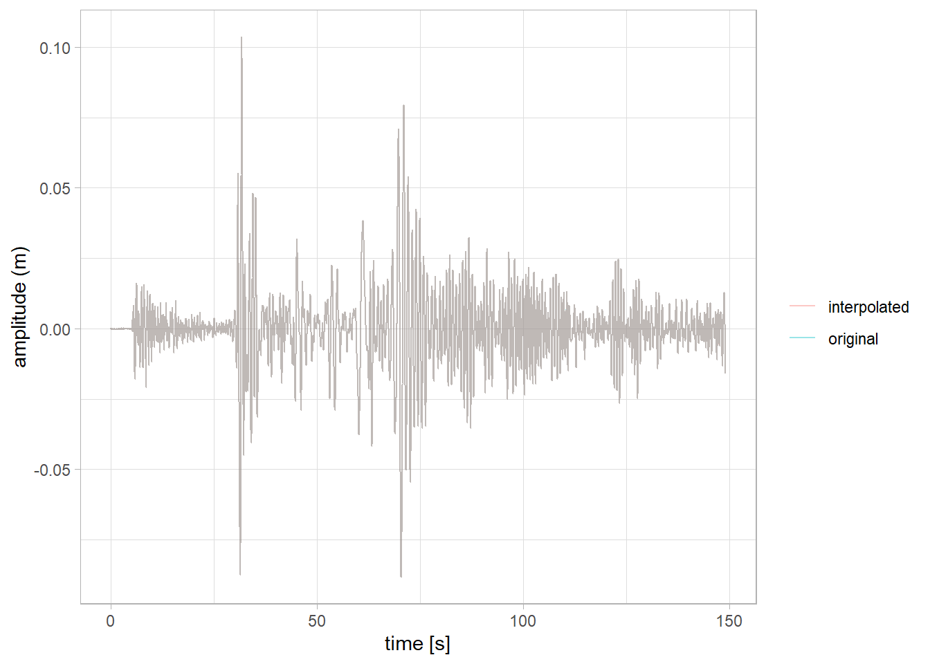
The two series are indistinguishable, so we are safe to proceed.
3.2.2 Lowpass filter
Let’s use a Butterworth filter with a cutoff_scale of 2 to remove all frequencies with a period of less than 2s. This is known as a low-pass filter.
fs <- 1000  # 1 kHz sampling rate
f_nyq <- fs / 2  # Nyquist frequency
f_cutoff <- 1/2  # 2s period

# Create Butterworth filter
butter_low <- butter(2, f_cutoff / f_nyq, type = "low")

# Apply filter
lp <- filtfilt(butter_low, coredata(ts_interp))

ggplot() +
  geom_line(data = data.frame(time = index(ts_interp), ground_motion = coredata(ts_interp)),
           aes(x = time, y = ground_motion, color = 'original')) +
  geom_line(data = data.frame(time = index(ts_interp), ground_motion = lp),
           aes(x = time, y = ground_motion, color = 'low-pass')) +
  labs(x = 'time [s]', y = 'amplitude (m)', color = '') +
  theme_light()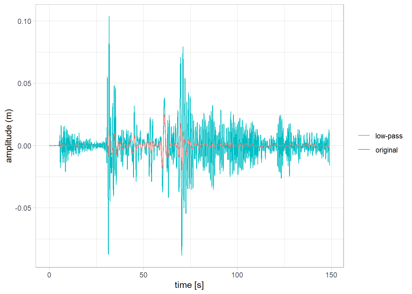
3.2.3 High-pass filter
The opposite operation is a high-pass filter, which keeps only frequencies higher than a given cutoff. To generate a high-pass filter, you can simply subtract the low-pass filtered version from the original:
hp <- coredata(ts_interp) - lp

ggplot() +
  geom_line(data = data.frame(time = index(ts_interp), ground_motion = coredata(ts_interp)),
           aes(x = time, y = ground_motion, color = 'original')) +
  geom_line(data = data.frame(time = index(ts_interp), ground_motion = hp),
           aes(x = time, y = ground_motion, color = 'high-pass'), alpha = 0.8) +
  labs(x = 'time [s]', y = 'amplitude (m)', color = '') +
  theme_light()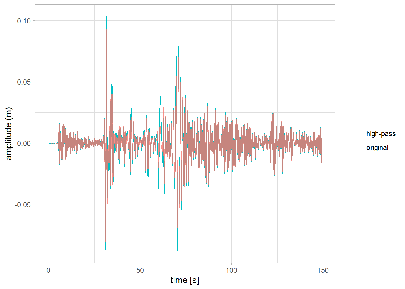
3.2.4 Band-pass filter
If you want to isolate variability in a band of frequencies (say 1-2s), you can create a band-pass filter:
f_low <- 1/2  # 2s period
f_high <- 1/1  # 1s period

butter_band <- butter(2, c(f_low, f_high) / f_nyq, type = "pass")
bp <- filtfilt(butter_band, coredata(ts_interp))

ggplot() +
  geom_line(data = data.frame(time = index(ts_interp), ground_motion = coredata(ts_interp)),
           aes(x = time, y = ground_motion, color = 'original')) +
  geom_line(data = data.frame(time = index(ts_interp), ground_motion = bp),
           aes(x = time, y = ground_motion, color = '1-2s band-pass'), alpha = 0.8) +
  labs(x = 'time [s]', y = 'amplitude (m)', color = '') +
  theme_light()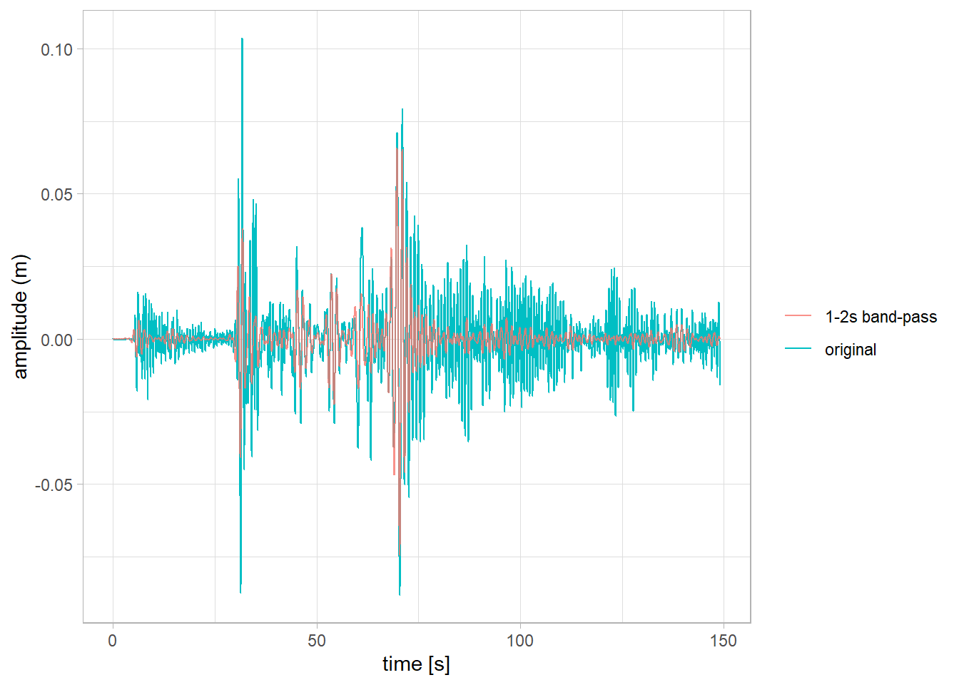
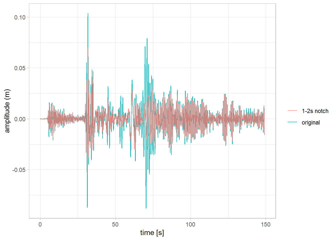
3.2.5 Notch filter
Conversely, if you wanted to remove all variability between 1-2s (a notch in frequency space), you would subtract the bandpass-filtered version.
notch <- coredata(ts_interp) - bp

ggplot() +
  geom_line(data = data.frame(time = index(ts_interp), ground_motion = coredata(ts_interp)),
           aes(x = time, y = ground_motion, color = 'original')) +
  geom_line(data = data.frame(time = index(ts_interp), ground_motion = notch),
           aes(x = time, y = ground_motion, color = '1-2s notch'), alpha = 0.8) +
  labs(x = 'time [s]', y = 'amplitude (m)', color = '') +
  theme_light()