2.2 Data Wrangling

2.2.1 Load packages

library(dplyr)
library(ggplot2)

2.2.2 Load data

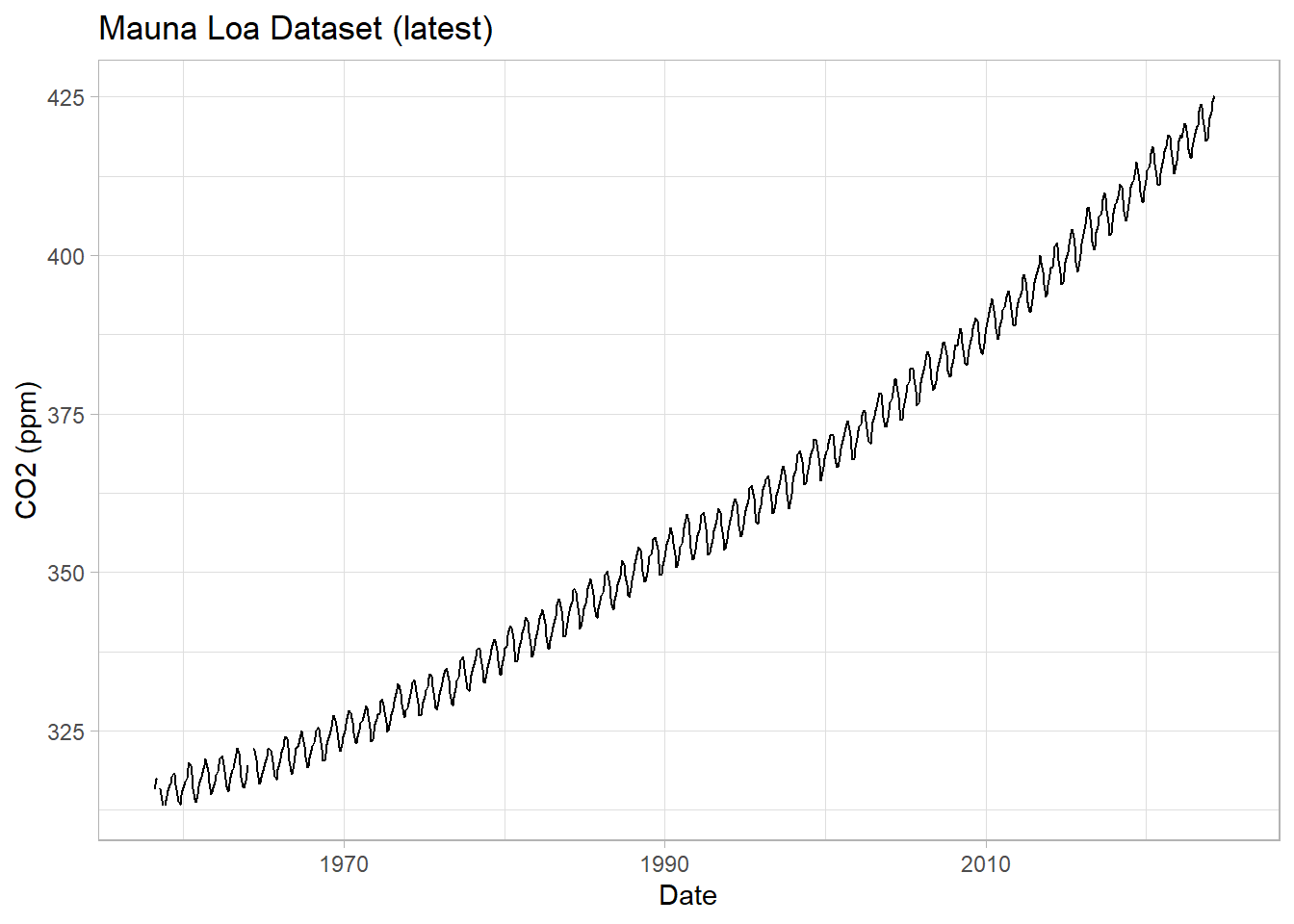
We can pull the data directly from the Scripps Institute website

df1 <- read.csv("https://scrippsco2.ucsd.edu/assets/data/atmospheric/stations/in_situ_co2/monthly/monthly_in_situ_co2_mlo.csv")

head(df1)

##   X...........................................................................................
## 1   Atmospheric CO2 concentrations (ppm) derived from in situ air measurements                
## 2   at Mauna Loa, Observatory, Hawaii: Latitude 19.5°N Longitude 155.6°W Elevation 3397m      
## 3   Since December 2022 sampling has temporarily been relocated to MaunuaKea, Hawaii          
## 4                                      Latitude 19.8°N Longitude 155.5°W Elevation 4145m      
## 5                                                                                             
## 6   Source: R. F. Keeling, S. J. Walker, S. C. Piper and A. F. Bollenbacher

Ooo, that doesn’t look right. This file has a big header, and doesn’t quite follow a normal spreadsheet format for the column headers. Let’s skip the header and column names. We can add them back in after loading.

df1 <- read.csv("https://scrippsco2.ucsd.edu/assets/data/atmospheric/stations/in_situ_co2/monthly/monthly_in_situ_co2_mlo.csv",skip=64,header = F)


head(df1)

##     V1 V2    V3       V4     V5     V6     V7     V8     V9    V10  V11
## 1 1958  1 21200 1958.041 -99.99 -99.99 -99.99 -99.99 -99.99 -99.99  MLO
## 2 1958  2 21231 1958.126 -99.99 -99.99 -99.99 -99.99 -99.99 -99.99  MLO
## 3 1958  3 21259 1958.203 315.71 314.44 316.20 314.91 315.71 314.44  MLO
## 4 1958  4 21290 1958.288 317.45 315.16 317.30 314.99 317.45 315.16  MLO
## 5 1958  5 21320 1958.370 317.51 314.69 317.89 315.07 317.51 314.69  MLO
## 6 1958  6 21351 1958.455 -99.99 -99.99 317.27 315.15 317.27 315.15  MLO

Okay, not the data looks right.

2.2.3 Format data

Lets add the column names.

names(df1) <- c('Yr','Mn','XLDate','Date','CO2','seasonally adjusted','fit','seasonally adjusted fit','CO2 filled','seasonally adjusted filled','Sta')
head(df1)

##     Yr Mn XLDate     Date    CO2 seasonally adjusted    fit seasonally adjusted fit
## 1 1958  1  21200 1958.041 -99.99              -99.99 -99.99                  -99.99
## 2 1958  2  21231 1958.126 -99.99              -99.99 -99.99                  -99.99
## 3 1958  3  21259 1958.203 315.71              314.44 316.20                  314.91
## 4 1958  4  21290 1958.288 317.45              315.16 317.30                  314.99
## 5 1958  5  21320 1958.370 317.51              314.69 317.89                  315.07
## 6 1958  6  21351 1958.455 -99.99              -99.99 317.27                  315.15
##   CO2 filled seasonally adjusted filled  Sta
## 1     -99.99                     -99.99  MLO
## 2     -99.99                     -99.99  MLO
## 3     315.71                     314.44  MLO
## 4     317.45                     315.16  MLO
## 5     317.51                     314.69  MLO
## 6     317.27                     315.15  MLO

The missing value default here is -99.99, let’s change that to NA, R’s standard.

df1 <- df1 %>% mutate(across(everything(), ~replace(., . ==  -99.99 , NA)))

2.2.4 First viz

Okay, we’re ready for an initial plot

ggplot(data=df1, mapping=aes(x=Date, y=CO2)) + 
  geom_line() +
  labs(title = "Mauna Loa Dataset (latest)",
       y="CO2 (ppm)") +
  theme_light()

Great, that looks right.