6.4 Wavelet Analysis

Lastly, we play with wavelet analysis, which may be used to “unfold” a spectrum and look at its evolution over time. There are several ways to access that functionality in Pyleoclim, but here we use summary_plot, which stacks together the timeseries itself, its scalogram (a plot of the magnitude of the wavelet power), and the power spectral density (PSD) obtained from summing the wavelet coefficients over time.

Age.interp <- seq(ceiling(min(dDdf$AgeKy)), floor(max(dDdf$AgeKy)), by=0.5)

df2 <- data.frame("AgeKy" = Age.interp,
        "Deuterium" = rep(NA, length(Age.interp)))

dDdf2 <- merge.data.frame(dDdf, df2, all = T)

dDdf3 <- dDdf2 %>%
  mutate(Temp.interp = approx(AgeKy, Temperature, AgeKy)$y) %>%
  mutate(D.interp = approx(AgeKy, Deuterium, AgeKy)$y) %>%
  dplyr::filter(AgeKy %in% Age.interp) %>%
  select(AgeKy, D.interp, Temp.interp) %>%
  rename(Age = AgeKy)

head(dDdf3)

##   Age  D.interp Temp.interp
## 1 1.0 -398.6369 -0.42737296
## 2 1.5 -398.3863 -0.40229635
## 3 2.0 -401.5101 -0.93168060
## 4 2.5 -394.8719  0.14813821
## 5 3.0 -395.7483 -0.01805415
## 6 3.5 -400.3498 -0.80095654

dDdf4 <- dDdf3 %>%
  select(-Temp.interp)

dD_wave <- biwavelet::wt(dDdf4, do.sig = F)

par(oma = c(0, 0, 0, 1), mar = c(5, 4, 4, 5) + 0.1)
plot(dD_wave, plot.cb=TRUE, plot.phase=FALSE)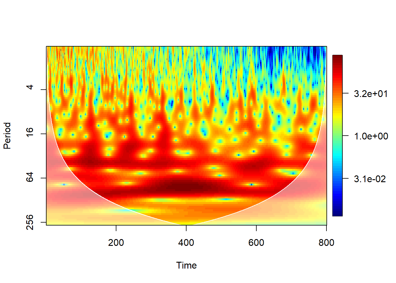

The scalogram reveals how spectral power (technically, wavelet power) changes over time. But which aspects of this are significant?

6.4.1 Null hypothesis

There are ways to test this using an AR(1) benchmark. Let’s use the conditional-sum-of-squares method to fit the AR1 model. (see ?arima for details)

dD_wave <- biwavelet::wt(dDdf4, do.sig = TRUE, arima.method = "CSS")

par(oma = c(0, 0, 0, 1), mar = c(5, 4, 4, 5) + 0.1)
plot(dD_wave, plot.cb=TRUE, plot.phase=FALSE)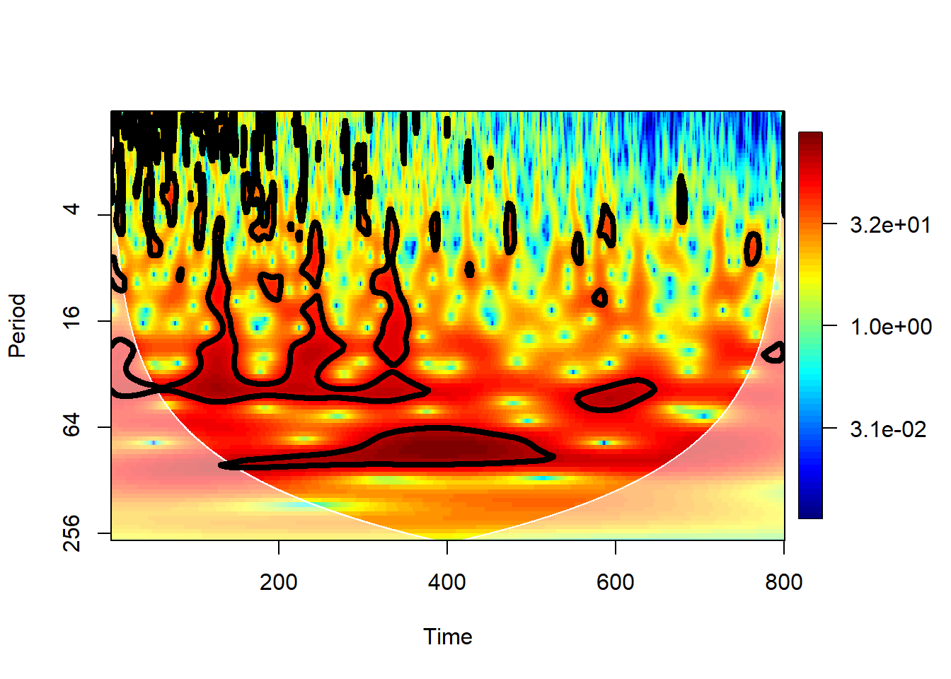

The solid lines delineate regions of the scalogram that are significant against an AR(1) benchmark, thus encircling “islands” of notable power. We see that the 100kyr periodicity is particularly pronounced around 300-600 kyr BP, while the 40 and 20kyr periodicities are more pronounced in the later portions (since 400 ky BP). This may be because of the compaction of the ice at depth, which you wouldn’t know from analyzing just this dataset. Paleoclimate timeseries must always be interpreted with those possible artifacts in mind. There are a lot of significant islands at short (<5ky) scales as well, but it is unclear whether this is reflective of large-scale climate variability.