6.5 Temperature vs CO2

Now let us load the CO2 composite from this and other neighboring sites around Antarctica:

co2df <- read.table('ftp://ftp.ncdc.noaa.gov/pub/data/paleo/icecore/antarctica/antarctica2015co2composite.txt', skip = 137, sep = "\t", header = T)
head(co2df)

##   age_gas_calBP co2_ppm co2_1s_ppm
## 1        -51.03  368.02       0.06
## 2        -48.00  361.78       0.37
## 3        -46.28  359.65       0.10
## 4        -44.41  357.11       0.16
## 5        -43.08  353.95       0.04
## 6        -42.31  353.72       0.22

We’ll again scale the Age column to kyr, and we’ll rename the verbose columns

co2df <- co2df %>%
  mutate(Age = age_gas_calBP/1000) %>%
  rename(CO2 = co2_ppm) %>%
  select(Age, CO2)

head(co2df)

##        Age    CO2
## 1 -0.05103 368.02
## 2 -0.04800 361.78
## 3 -0.04628 359.65
## 4 -0.04441 357.11
## 5 -0.04308 353.95
## 6 -0.04231 353.72

Let’s have a look

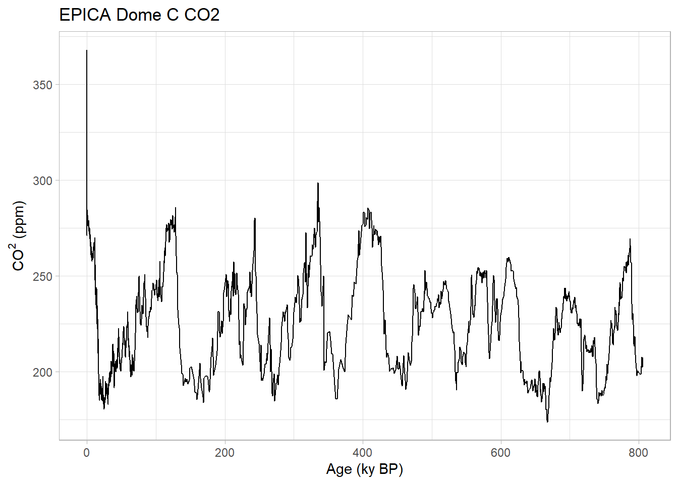
ggplot(data = co2df, mapping=aes(x=Age, y=CO2)) + 
  geom_line() +
  labs(title = "EPICA Dome C CO2",
       x="Age (ky BP)",
       y=expression(paste(CO^2, " (ppm)", sep=""))) +
  theme_light()