Downsampling — Simulating Sparse Proxy Records

Author

Jordan Landers

Published

June 12, 2026

Abstract

resample.downsample sub-samples a regularly spaced model trajectory to simulate the irregular sampling of paleoclimate proxy records. This notebook demonstrates four gap-distribution modes — exponential, Poisson, Pareto, and random_choice — and shows how to inspect the resulting resolution statistics using pyleoclim’s resolution dashboard.

Keywords

downsample, sub-sampling, proxy records, sparse sampling, exponential, Poisson, Pareto, random_choice, resolution, pyleoclim

import numpy as np
import matplotlib.pyplot as plt
import pyleoclim as pyleo
from climatecritters.utils.resample import downsample

series = pyleo.utils.load_dataset('SOI').interp()
print(f'n={len(series.time)}  dt={series.time[1]-series.time[0]:.3f} yr  '
      f'span={series.time[0]:.1f}–{series.time[-1]:.1f} yr')

n=1909  dt=0.083 yr  span=1866.0–2025.0 yr
{'archiveType': 'Instrumental', 'label': 'Southern Oscillation Index'}

Original series and resolution

fig, ax = series.plot()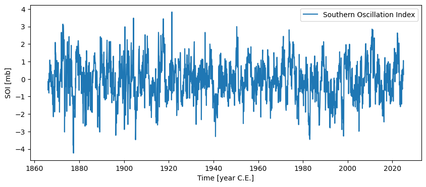

{'archiveType': 'Instrumental', 'label': 'Southern Oscillation Index'}

series.resolution().dashboard()

(<Figure size 1100x800 with 2 Axes>,
 {'res': <Axes: xlabel='Time [year C.E.]', ylabel='resolution [year C.E.]'>,
  'res_hist': <Axes: xlabel='Counts'>})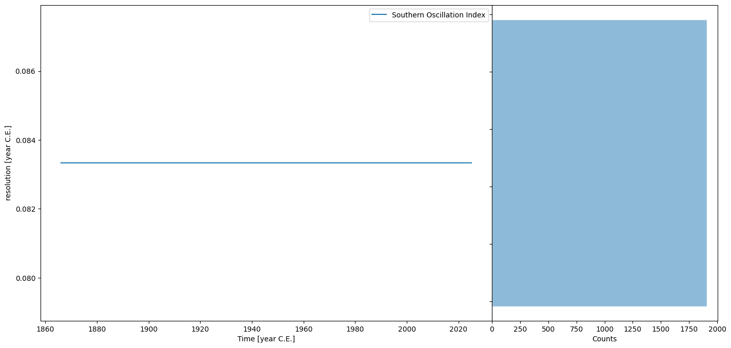

{'archiveType': 'Instrumental', 'label': 'Southern Oscillation Index'}

Exponential

method='exponential', param=[scale]

Index gaps ~ Exponential(scale). Scale = mean gap size. Heavy right tail: most gaps are small, occasional large ones — like bioturbated marine records.

ds_exp = downsample(series, method='exponential', param=[2], seed=42)

{'archiveType': 'Instrumental', 'label': 'Southern Oscillation Index'}
{'archiveType': 'Instrumental', 'label': 'Southern Oscillation Index'}

fig, ax = plt.subplots(figsize=(11, 3))
ax.plot(series.time, series.value,
        color='#888888', lw=1.0, alpha=0.6, label='original')
ax.plot(ds_exp.time, ds_exp.value,
        color='#2196F3', lw=1.5, alpha=0.9, label='downsampled')
ax.set_ylabel('SOI'); ax.legend(fontsize=9)
plt.tight_layout(); plt.show()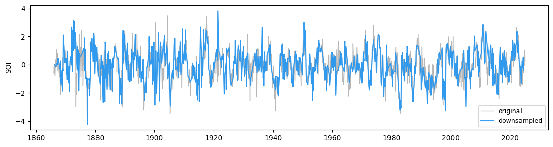

{'archiveType': 'Instrumental', 'label': 'Southern Oscillation Index'}
{'archiveType': 'Instrumental', 'label': 'Southern Oscillation Index'}

Figure. The sparse record (blue) keeps exact values at selected indices. Compare coverage and gap structure to the original (gray).

ds_exp.resolution().dashboard()

(<Figure size 1100x800 with 2 Axes>,
 {'res': <Axes: xlabel='Time [year C.E.]', ylabel='resolution [year C.E.]'>,
  'res_hist': <Axes: xlabel='Counts'>})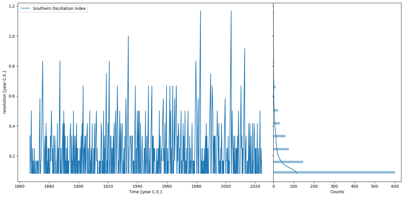

{'archiveType': 'Instrumental', 'label': 'Southern Oscillation Index'}
{'archiveType': 'Instrumental', 'label': 'Southern Oscillation Index'}

Poisson

method='poisson', param=[rate]

Gaps ~ Poisson(rate) + 1. More symmetric around the mean — fewer extreme long gaps than Exponential.

ds_poi = downsample(series, method='poisson', param=[3], seed=42)

{'archiveType': 'Instrumental', 'label': 'Southern Oscillation Index'}
{'archiveType': 'Instrumental', 'label': 'Southern Oscillation Index'}
{'archiveType': 'Instrumental', 'label': 'Southern Oscillation Index'}

fig, ax = plt.subplots(figsize=(11, 3))
ax.plot(series.time, series.value,
        color='#888888', lw=1.0, alpha=0.6, label='original')
ax.plot(ds_poi.time, ds_poi.value,
        color='#E91E63', lw=1.5, alpha=0.9, label='downsampled')
ax.set_ylabel('SOI'); ax.legend(fontsize=9)
plt.tight_layout(); plt.show()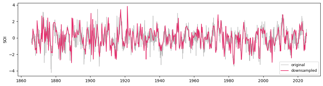

{'archiveType': 'Instrumental', 'label': 'Southern Oscillation Index'}
{'archiveType': 'Instrumental', 'label': 'Southern Oscillation Index'}
{'archiveType': 'Instrumental', 'label': 'Southern Oscillation Index'}

Figure. Tighter gap distribution: coverage is more uniform than Exponential, fewer long stretches without a sample.

ds_poi.resolution().dashboard()

(<Figure size 1100x800 with 2 Axes>,
 {'res': <Axes: xlabel='Time [year C.E.]', ylabel='resolution [year C.E.]'>,
  'res_hist': <Axes: xlabel='Counts'>})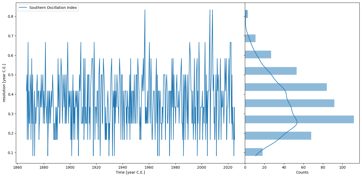

{'archiveType': 'Instrumental', 'label': 'Southern Oscillation Index'}
{'archiveType': 'Instrumental', 'label': 'Southern Oscillation Index'}
{'archiveType': 'Instrumental', 'label': 'Southern Oscillation Index'}

Pareto

method='pareto', param=[shape, scale]

Gaps ~ (Pareto(shape) + 1) × scale. Power-law tail: small shape → very heavy tail with occasional extremely long hiatuses. Mimics patchy carbonate preservation.

ds_par = downsample(series, method='pareto', param=[2, 1], seed=42)

{'archiveType': 'Instrumental', 'label': 'Southern Oscillation Index'}
{'archiveType': 'Instrumental', 'label': 'Southern Oscillation Index'}
{'archiveType': 'Instrumental', 'label': 'Southern Oscillation Index'}
{'archiveType': 'Instrumental', 'label': 'Southern Oscillation Index'}

fig, ax = plt.subplots(figsize=(11, 3))
ax.plot(series.time, series.value,
        color='#888888', lw=1.0, alpha=0.6, label='original')
ax.plot(ds_par.time, ds_par.value,
        color='#4CAF50', lw=1.5, alpha=0.9, label='downsampled')
ax.set_ylabel('SOI'); ax.legend(fontsize=9)
plt.tight_layout(); plt.show()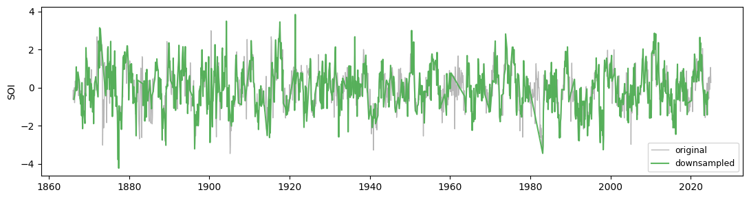

{'archiveType': 'Instrumental', 'label': 'Southern Oscillation Index'}
{'archiveType': 'Instrumental', 'label': 'Southern Oscillation Index'}
{'archiveType': 'Instrumental', 'label': 'Southern Oscillation Index'}
{'archiveType': 'Instrumental', 'label': 'Southern Oscillation Index'}

Figure. Rare but very long gaps dominate the resolution dashboard — the heavy tail means the record can go silent for extended periods.

ds_par.resolution().dashboard()

(<Figure size 1100x800 with 2 Axes>,
 {'res': <Axes: xlabel='Time [year C.E.]', ylabel='resolution [year C.E.]'>,
  'res_hist': <Axes: xlabel='Counts'>})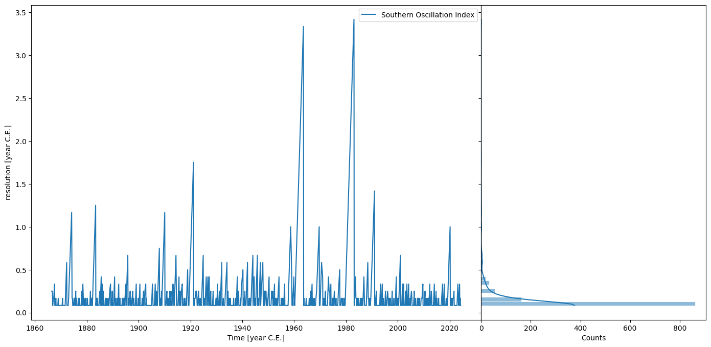

{'archiveType': 'Instrumental', 'label': 'Southern Oscillation Index'}
{'archiveType': 'Instrumental', 'label': 'Southern Oscillation Index'}
{'archiveType': 'Instrumental', 'label': 'Southern Oscillation Index'}
{'archiveType': 'Instrumental', 'label': 'Southern Oscillation Index'}

Random choice

method='random_choice', param=[[values], [probabilities]]

Gaps drawn from a discrete distribution. Use when you know the sampling process — e.g. annual cores with occasional multi-year losses.

ds_rc = downsample(series, method='random_choice',
                   param=[[1, 5, 20], [0.80, 0.15, 0.05]], seed=42)

{'archiveType': 'Instrumental', 'label': 'Southern Oscillation Index'}
{'archiveType': 'Instrumental', 'label': 'Southern Oscillation Index'}
{'archiveType': 'Instrumental', 'label': 'Southern Oscillation Index'}
{'archiveType': 'Instrumental', 'label': 'Southern Oscillation Index'}
{'archiveType': 'Instrumental', 'label': 'Southern Oscillation Index'}

fig, ax = plt.subplots(figsize=(11, 3))
ax.plot(series.time, series.value,
        color='#888888', lw=1.0, alpha=0.6, label='original')
ax.plot(ds_rc.time, ds_rc.value,
        color='#9C27B0', lw=1.5, alpha=0.9, label='downsampled')
ax.set_ylabel('SOI'); ax.legend(fontsize=9)
plt.tight_layout(); plt.show()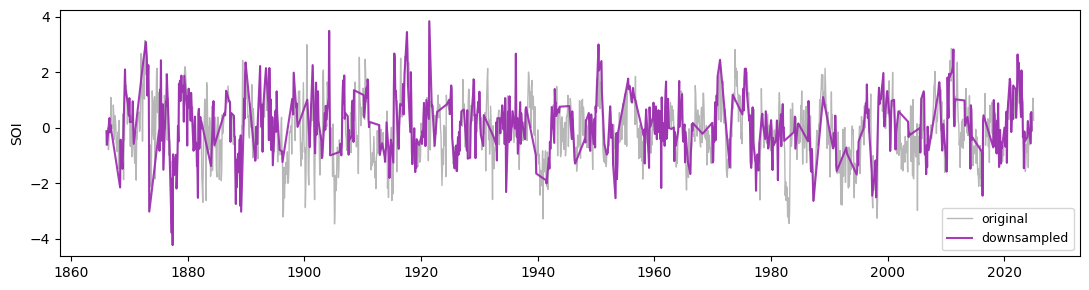

{'archiveType': 'Instrumental', 'label': 'Southern Oscillation Index'}
{'archiveType': 'Instrumental', 'label': 'Southern Oscillation Index'}
{'archiveType': 'Instrumental', 'label': 'Southern Oscillation Index'}
{'archiveType': 'Instrumental', 'label': 'Southern Oscillation Index'}
{'archiveType': 'Instrumental', 'label': 'Southern Oscillation Index'}

Figure. Three distinct gap sizes visible in the resolution dashboard, at the specified probabilities (80 % × 1, 15 % × 5, 5 % × 20).

ds_rc.resolution().dashboard()

(<Figure size 1100x800 with 2 Axes>,
 {'res': <Axes: xlabel='Time [year C.E.]', ylabel='resolution [year C.E.]'>,
  'res_hist': <Axes: xlabel='Counts'>})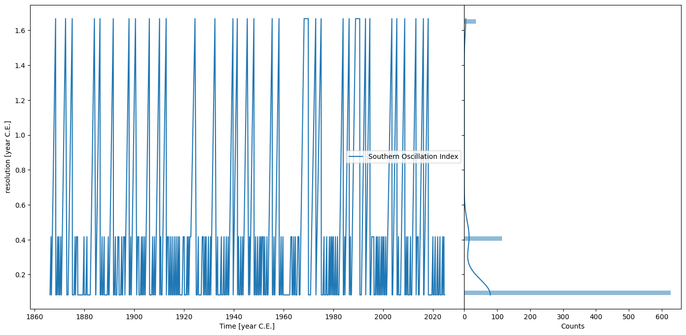

{'archiveType': 'Instrumental', 'label': 'Southern Oscillation Index'}
{'archiveType': 'Instrumental', 'label': 'Southern Oscillation Index'}
{'archiveType': 'Instrumental', 'label': 'Southern Oscillation Index'}
{'archiveType': 'Instrumental', 'label': 'Southern Oscillation Index'}
{'archiveType': 'Instrumental', 'label': 'Southern Oscillation Index'}

Method comparison — gap-size histograms

labels  = ['Exponential(2)', 'Poisson(3)', 'Pareto(2,1)', 'RC(1/5/20)']
dss     = [ds_exp, ds_poi, ds_par, ds_rc]
colours = ['#2196F3', '#E91E63', '#4CAF50', '#9C27B0']

fig, axes = plt.subplots(1, 4, figsize=(14, 4), sharey=True)
for ax, ds, lbl, col in zip(axes, dss, labels, colours):
    gaps = np.diff(ds.time)
    ax.hist(gaps, bins=30, color=col, alpha=0.7, edgecolor='none')
    ax.axvline(gaps.mean(), color='k', lw=1.2, ls='--',
               label=f'mean={gaps.mean():.2f}')
    ax.set_title(lbl, fontsize=9); ax.set_xlabel('Δt'); ax.legend(fontsize=7)
axes[0].set_ylabel('count')
fig.suptitle('Gap-size histograms for all four methods')
plt.tight_layout(); plt.show()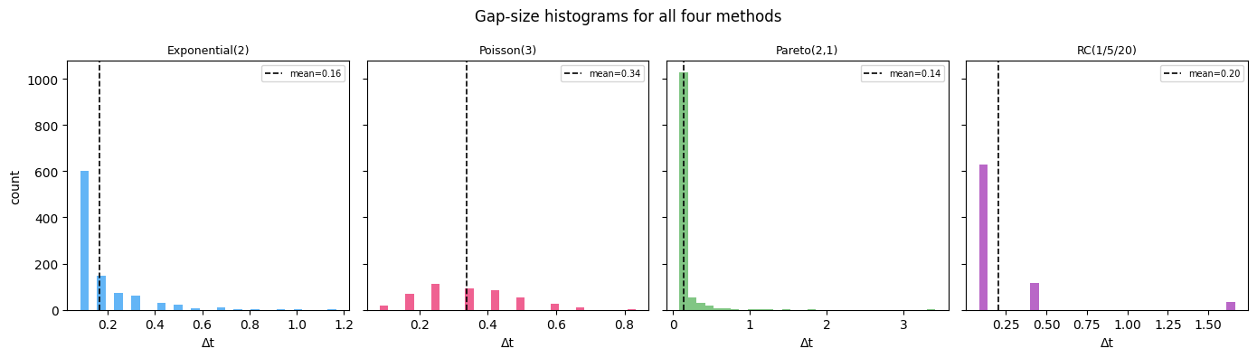

{'archiveType': 'Instrumental', 'label': 'Southern Oscillation Index'}
{'archiveType': 'Instrumental', 'label': 'Southern Oscillation Index'}
{'archiveType': 'Instrumental', 'label': 'Southern Oscillation Index'}
{'archiveType': 'Instrumental', 'label': 'Southern Oscillation Index'}
{'archiveType': 'Instrumental', 'label': 'Southern Oscillation Index'}
{'archiveType': 'Instrumental', 'label': 'Southern Oscillation Index'}
{'archiveType': 'Instrumental', 'label': 'Southern Oscillation Index'}
{'archiveType': 'Instrumental', 'label': 'Southern Oscillation Index'}
{'archiveType': 'Instrumental', 'label': 'Southern Oscillation Index'}
{'archiveType': 'Instrumental', 'label': 'Southern Oscillation Index'}

Figure. Exponential: mode near zero, exponential decay. Poisson: symmetric around the mean. Pareto: heavy right tail. Random choice: discrete spikes at the specified values. Choose the distribution that matches your sampling process.