ENSORechargeOscillator — Jin (1997) ENSO Recharge Paradigm

Author

Jordan Landers

Published

June 12, 2026

Abstract

ENSORechargeOscillator implements Jin’s (1997) recharge-discharge paradigm, coupling SST anomaly T to thermocline depth anomaly h to produce El Niño/La Niña oscillations. This notebook explores damped, self-sustained, and nonlinear oscillation regimes controlled by Bjerknes coupling μ, and shows how seasonal forcing can entrain the oscillator into irregular, quasi-periodic behavior.

Keywords

ENSORechargeOscillator, ENSO, recharge-discharge, Bjerknes coupling, thermocline, SST anomaly, limit cycle, seasonal forcing, nonlinear damping, Jin 1997

Overview

ENSORechargeOscillator implements the Jin (1997) recharge-discharge paradigm coupling the eastern Pacific SST anomaly T to the thermocline depth anomaly h:

\[\frac{dT}{dt} = R\,T + \gamma\,h - \epsilon_n(h + b\,T)^3 + F(t)\]

\[\frac{dh}{dt} = -r\,h - \alpha\,b\,T\]

where \(b = b_0\mu\) (Bjerknes coupling) and \(R = \gamma b - c\) (net SST tendency).

The model spans three dynamical regimes controlled primarily by mu (Bjerknes coupling): - Damped oscillator (mu below critical): perturbations decay, ENSO needs external forcing to oscillate - Limit cycle (mu near/above critical): self-sustained oscillations without seasonal forcing - Nonlinear regime (en > 0): cubic damping limits amplitude growth

Parameters

Name	Description	Default
`mu`	Bjerknes coupling coefficient	0.7
`en`	Nonlinear damping	0.0
`c`	Newtonian SST cooling rate	1.0
`r`	Thermocline recharge damping	0.25
`alpha`	Wind-stress feedback	0.125
`b0`	Background thermocline slope sensitivity	2.5
`gamma`	Thermocline feedback onto SST	0.75

Time units: months by convention. Seasonal forcing is added externally via register_forcing. State variables: T (SST anomaly, °C), h (thermocline depth anomaly, m).

import numpy as np
import matplotlib.pyplot as plt
import climatecritters as cc
from climatecritters.model_critters.enso_recharge import ENSORechargeOscillator
from climatecritters.utils.forcing import create_sinusoid_forcing

Unforced dynamics: μ regimes

Without seasonal forcing, the linear stability of the steady state \((T, h) = (0, 0)\) depends on mu. The critical coupling \(\mu_c\) separates damped oscillations from spontaneous limit-cycle growth.

mu_cases = [
    (0.5, 'Damped  (mu=0.5)',           'steelblue'),
    (0.7, 'Near-critical  (mu=0.7)',    'goldenrod'),
    (0.9, 'Self-sustained  (mu=0.9)',   'firebrick'),
]

fig, axes = plt.subplots(2, 1, figsize=(11, 6), sharex=True)

for mu_val, label, color in mu_cases:
    m = ENSORechargeOscillator(mu=mu_val)
    out = m.integrate(t_span=(0, 240), y0=[0.5, 0.0], method='RK45')
    t = np.asarray(out.time)
    axes[0].plot(t, out.state_variables['T'], lw=1.0, color=color, label=label)
    axes[1].plot(t, out.state_variables['h'], lw=1.0, color=color)

axes[0].axhline(0, color='k', lw=0.4, ls='--')
axes[0].set_ylabel('T  (SST anomaly)'); axes[0].set_title('SST anomaly T')
axes[0].legend(fontsize=9)

axes[1].axhline(0, color='k', lw=0.4, ls='--')
axes[1].set_ylabel('h  (thermocline depth)'); axes[1].set_xlabel('time (months)')
axes[1].set_title('Thermocline depth anomaly h')

fig.suptitle('ENSORechargeOscillator — unforced, varying mu')
plt.tight_layout(); plt.show()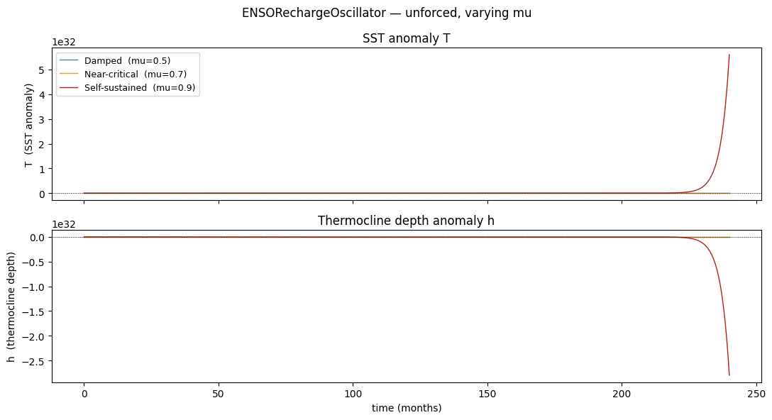

Figure. Top: SST anomaly \(T(t)\) for three coupling strengths. At \(\mu=0.5\) the oscillation decays — ENSO is subcritical and needs external forcing to persist. At \(\mu=0.7\) weak self-sustained oscillations emerge near the critical point. At \(\mu=0.9\) the system is supercritical: a growing limit cycle with multi-year ENSO swings. Bottom: thermocline anomaly \(h\) lags \(T\) by roughly a quarter period — thermocline recharge precedes each El Niño peak.

Phase portrait: T vs h

The recharge oscillator has a clear physical interpretation in the T–h plane: - El Niño events: warm T + positive h (thermocline high → enhanced SST feedback) - Discharge phase: warm T drives negative h tendency (recharge → discharge) - La Niña events: cold T + negative h - Recharge phase: cold T drives positive h tendency

# Long run for the self-sustained case (mu=0.9)
m_lc = ENSORechargeOscillator(mu=0.9)
out_lc = m_lc.integrate(t_span=(0, 600), y0=[0.5, 0.0], method='RK45')
t_lc = np.asarray(out_lc.time)
T_lc = out_lc.state_variables['T']
h_lc = out_lc.state_variables['h']
mask_lc = t_lc > 100   # discard transient

fig, axes = plt.subplots(1, 2, figsize=(12, 4))

sc = axes[0].scatter(T_lc[mask_lc], h_lc[mask_lc], c=t_lc[mask_lc], cmap='plasma',
                     s=2, lw=0)
fig.colorbar(sc, ax=axes[0], label='time (months)')
axes[0].axhline(0, color='k', lw=0.4, ls='--')
axes[0].axvline(0, color='k', lw=0.4, ls='--')
axes[0].set_xlabel('T (SST anomaly)'); axes[0].set_ylabel('h (thermocline)')
axes[0].set_title('Phase portrait — limit cycle  (mu=0.9)')

# Annotate quadrants
for txt, xy in [('El Niño\n(warm, high h)', (1.2, 1.0)),
                ('La Niña\n(cold, low h)',  (-1.6, -0.8))]:
    axes[0].text(*xy, txt, fontsize=7.5, ha='center', style='italic', color='#555555')

axes[1].plot(t_lc[mask_lc], T_lc[mask_lc], lw=0.8, color='firebrick')
axes[1].axhline(0, color='k', lw=0.4, ls='--')
axes[1].set_xlabel('time (months)'); axes[1].set_ylabel('T')
axes[1].set_title('T(t) — self-sustained ENSO cycle')

fig.suptitle('ENSORechargeOscillator — mu=0.9, unforced')
plt.tight_layout(); plt.show()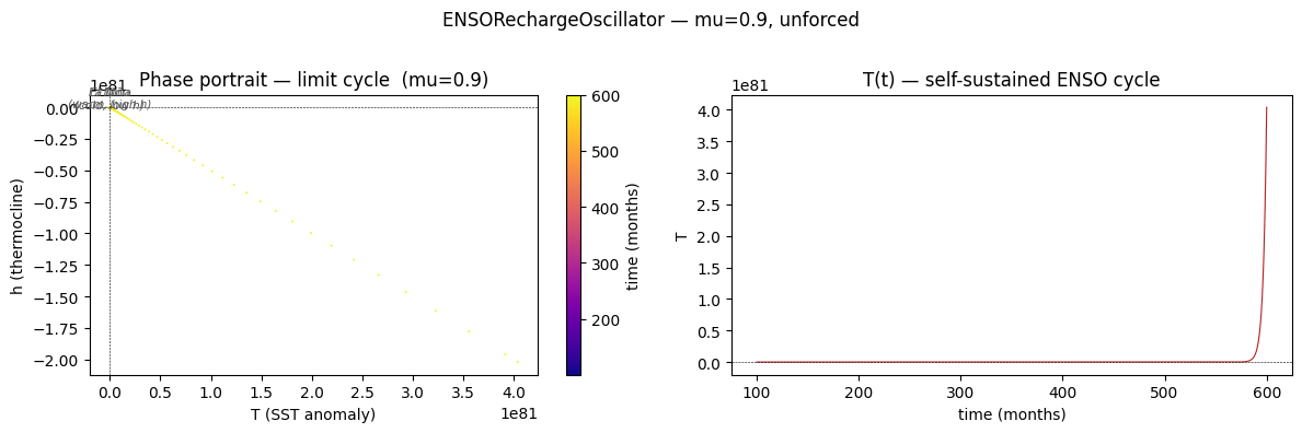

Figure. Left: T–h phase portrait of the self-sustained limit cycle (\(\mu=0.9\)), coloured by time. The cycle runs clockwise: warm \(T\) (El Niño peak, top-right) discharges the thermocline, driving the system toward La Niña (bottom-left), which then recharges. Right: \(T(t)\) in the sustained regime shows quasi-regular ~4-year oscillations.

Seasonal forcing

Seasonal (or any other) external forcing is added via register_forcing with the create_sinusoid_forcing factory helper (additive, pre-step):

model = ENSORechargeOscillator(mu=0.7)
model.register_forcing(
    'T',
    create_sinusoid_forcing(A=0.5, period=6.0),
    attachment_style='additive',
    timing='pre',
)

# Damped oscillator (mu=0.5) with and without seasonal forcing
m_no_seas = ENSORechargeOscillator(mu=0.5)
out_no_seas = m_no_seas.integrate(t_span=(0, 240), y0=[0.5, 0.0], method='RK45')

m_seas = ENSORechargeOscillator(mu=0.5)
m_seas.register_forcing(
    'T',
    create_sinusoid_forcing(A=0.5, period=6.0),
    attachment_style='additive',
    timing='pre',
)
out_seas = m_seas.integrate(t_span=(0, 240), y0=[0.5, 0.0], method='RK45')

t_ns = np.asarray(out_no_seas.time)
t_s  = np.asarray(out_seas.time)

fig, axes = plt.subplots(2, 1, figsize=(11, 6), sharex=True)

axes[0].plot(t_ns, out_no_seas.state_variables['T'], color='steelblue', lw=1.0,
             label='No forcing — decays')
axes[0].plot(t_s,  out_seas.state_variables['T'],    color='firebrick',  lw=1.0,
             label='Seasonal forcing (A=0.5) — sustained')
axes[0].axhline(0, color='k', lw=0.4, ls='--')
axes[0].set_ylabel('T'); axes[0].set_title('SST anomaly')
axes[0].legend(fontsize=9)

# Show the seasonal forcing itself
t_fine = np.linspace(0, 240, 2000)
forcing_vals = 0.5 * np.sin(2 * np.pi * t_fine / 6.0)
axes[1].plot(t_fine, forcing_vals, color='goldenrod', lw=1.0)
axes[1].axhline(0, color='k', lw=0.4, ls='--')
axes[1].set_ylabel('Seasonal forcing'); axes[1].set_xlabel('time (months)')
axes[1].set_title('Seasonal forcing A·sin(2πt/period)  (A=0.5, period=6 months)')

fig.suptitle('ENSORechargeOscillator — damped case (mu=0.5) with/without seasonal forcing')
plt.tight_layout(); plt.show()

Figure. Top: with no seasonal forcing (\(\mu=0.5\)) the SST oscillation decays within ~5 years. Adding a 6-month sinusoidal kick (\(A_f=0.5\)) locks the system into a sustained, quasi-regular oscillation — the damped ENSO mode is entrained by the seasonal cycle. Bottom: the seasonal forcing itself.

Nonlinear damping

The cubic term \(-\epsilon_n(h + bT)^3\) limits amplitude growth in the supercritical regime. Without it a large mu gives unbounded growth; with en > 0 the system settles onto a finite-amplitude limit cycle.

en_cases = [
    (0.0,  'en=0  (linear)',       'firebrick'),
    (0.05, 'en=0.05  (weak nl.)',  'goldenrod'),
    (0.2,  'en=0.2  (strong nl.)', 'steelblue'),
]

fig, ax = plt.subplots(figsize=(10, 4))

for en_val, label, color in en_cases:
    m = ENSORechargeOscillator(mu=0.9, en=en_val)
    out = m.integrate(t_span=(0, 300), y0=[0.5, 0.0], method='RK45')
    t = np.asarray(out.time)
    ax.plot(t, out.state_variables['T'], lw=0.9, color=color, label=label)

ax.axhline(0, color='k', lw=0.4, ls='--')
ax.set_xlabel('time (months)'); ax.set_ylabel('T')
ax.set_title('Effect of nonlinear damping  (mu=0.9)')
ax.legend(fontsize=9)
plt.tight_layout(); plt.show()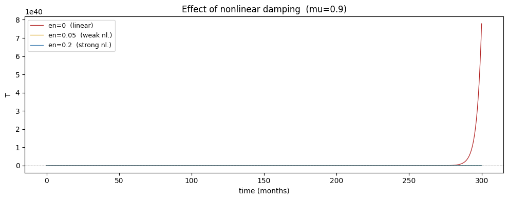

Figure. Effect of cubic damping on the supercritical case (\(\mu=0.9\)). Without damping (\(\epsilon_n=0\)) amplitude grows without bound. Weak damping (\(\epsilon_n=0.05\)) limits growth to a large but finite limit cycle. Strong damping (\(\epsilon_n=0.2\)) produces a compact, nearly sinusoidal cycle — the model’s analogue of amplitude-limited ENSO variability.

Solver notes

RK45 is appropriate. The system is not stiff at default parameters.

uses_post_history=True — diagnostics are assembled after integration. There are no diagnostic variables by default; state_variables contains T and h directly.

Time units are months by convention: t_span=(0, 120) is a 10-year run. A period of 6.0 is a semi-annual cycle; use period=12.0 for an annual cycle.

Seasonal forcing via register_forcing uses attachment_style='additive' and timing='pre' to add the seasonal signal before the tendency is computed:

model.register_forcing(
    'T',
    create_sinusoid_forcing(A=0.5, period=6.0),
    attachment_style='additive',
    timing='pre',
)

The create_sinusoid_forcing factory returns a plain callable f(t), so no partial wrapping is needed.