TwoBoxCarbon and BoxModelSpec — Carbon Cycle Box Models

Abstract

This notebook demonstrates two approaches to building carbon cycle box models. TwoBoxCarbon is a concrete two-reservoir model tracking atmospheric and surface-ocean carbon inventories via concentration-gradient exchange. BoxModelSpec provides a declarative framework for assembling arbitrary box networks using exchange and transport links, enabling three-box and more complex topologies without subclassing.

Keywords

TwoBoxCarbon, BoxModelSpec, carbon cycle, box model, air-sea exchange, concentration gradient, mass conservation, biological pump, network topology, declarative

import numpy as np
import matplotlib.pyplot as plt
import climatecritters as cc
from climatecritters.model_critters.two_box_carbon import TwoBoxCarbon
from climatecritters.model_critters.box_model import BoxModelSpec

TwoBoxCarbon

Closed system: mass conservation

With R=0 and l_s=0 the system is closed: total carbon A + S must remain constant to numerical precision. This checks that the concentration-gradient exchange (not raw inventory difference) conserves mass correctly even when V_atm ≠ V_surf.

# Closed system: V_atm ≪ V_surf — atmosphere equilibrates to surface ocean concentration
model_closed = TwoBoxCarbon(k=0.2, R=0.0, l_s=0.0, V_atm=1.0, V_surf=50.0)
out_closed = model_closed.integrate(t_span=(0, 100), y0=[100.0, 200.0], method='RK45')

A_c = out_closed.state_variables['A']
S_c = out_closed.state_variables['S']
total = A_c + S_c

print(f'Initial total: {total[0]:.6f}')
print(f'Final   total: {total[-1]:.6f}')
print(f'Max drift:     {np.max(np.abs(total - total[0])):.2e}  (numerical precision)')

Initial total: 300.000000
Final   total: 300.000000
Max drift:     1.71e-13  (numerical precision)

t_c = np.asarray(out_closed.time)

fig, ax = plt.subplots(figsize=(9, 4))
ax.plot(t_c, A_c, color='steelblue', lw=1.2, label='A (atmosphere)')
ax.plot(t_c, S_c, color='firebrick', lw=1.2, label='S (surface ocean)')
ax.plot(t_c, total, 'k--', lw=1.0, label='A + S (conserved)')
ax.set_xlabel('time'); ax.set_ylabel('carbon inventory')
ax.set_title('TwoBoxCarbon — closed system, V_atm=1, V_surf=50')
ax.legend()
plt.tight_layout(); plt.show()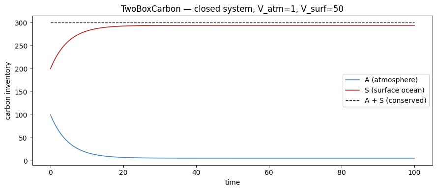

Figure. Both inventories relax toward a shared equilibrium concentration (\(A/V_{\rm atm} = S/V_{\rm surf}\)). Because \(V_{\rm surf} = 50 \times V_{\rm atm}\), the atmosphere ends up with roughly 1/51 of the total carbon. The dashed A + S line is flat to floating-point precision throughout.

Forced case: time-varying carbon source

A step-on/step-off pulse in R simulates an emission event. Registered via register_forcing so it is time-varying.

# Pulse: R=1 for 0 ≤ t < 30, then R=0 (atmosphere relaxes back)
pulse = cc.Forcing(lambda t: 1.0 if t < 30.0 else 0.0)

model_forced = TwoBoxCarbon(k=0.2, l_s=0.05, V_atm=1.0, V_surf=1.0)
model_forced.register_forcing('R', pulse)
out_forced = model_forced.integrate(t_span=(0, 150), y0=[0.0, 0.0], method='RK45')

t_f = np.asarray(out_forced.time)

fig, axes = plt.subplots(3, 1, figsize=(10, 7), sharex=True)

# Forcing
axes[0].step(t_f, [pulse.get_forcing(tt) for tt in t_f], where='post',
             color='goldenrod', lw=1.2)
axes[0].set_ylabel('R  (carbon/time)'); axes[0].set_title('Carbon source pulse')

# State variables
axes[1].plot(t_f, out_forced.state_variables['A'], color='steelblue', lw=1.2, label='A')
axes[1].plot(t_f, out_forced.state_variables['S'], color='firebrick', lw=1.2, label='S')
axes[1].set_ylabel('inventory'); axes[1].set_title('A and S inventories')
axes[1].legend()

# Net flux
axes[2].plot(t_f, out_forced.diagnostic_variables['net_flux'], color='purple', lw=1.0)
axes[2].axhline(0, color='k', lw=0.5, ls='--')
axes[2].set_ylabel('dA/dt'); axes[2].set_title('Net atmospheric flux (→ 0 at steady state)')
axes[2].set_xlabel('time')

fig.suptitle('TwoBoxCarbon — step-on/step-off carbon pulse')
plt.tight_layout(); plt.show()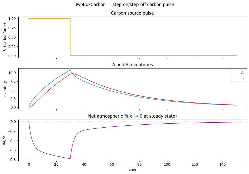

Figure. Top: step forcing pulse (\(R=1\) for \(t<30\), then off). Middle: \(A\) rises during the pulse then decays as air-sea exchange transfers carbon to the ocean; \(S\) follows with a slight lag and retains most of the perturbation. Bottom: net atmospheric flux is positive (net source) during the pulse, then negative (net uptake by ocean) during relaxation.

BoxModelSpec

Declarative rebuild of TwoBoxCarbon

BoxModelSpec lets you define the same equations without subclassing CCModel. Register state variables, parameters, tendency relations, and diagnostics; call make_boxmodel() to get an integrable model.

The spec below reproduces TwoBoxCarbon exactly — outputs match to floating-point precision.

spec = BoxModelSpec('two_box_carbon_generic')
spec.register_state_variables(['A', 'S'])
spec.register_diagnostic_variables(['net_flux'])
spec.register_parameters(k=0.2, R=0.0, l_s=0.05, V_atm=1.0, V_surf=1.0)
spec.register_input('R', fallback_param='R')   # R can be overridden by register_forcing

def exchange_flux(ctx):
    return ctx.param('k') * (ctx['A'] / ctx.param('V_atm') - ctx['S'] / ctx.param('V_surf'))

spec.register_relations({
    'A': lambda ctx: -exchange_flux(ctx) + ctx.input('R') - ctx.param('l_s') * ctx['A'],
    'S': lambda ctx:  exchange_flux(ctx),
})
spec.register_diagnostic(
    'net_flux',
    lambda ctx: -exchange_flux(ctx) + ctx.input('R') - ctx.param('l_s') * ctx['A'],
)

model_generic = spec.make_boxmodel()
model_generic.register_forcing('R', pulse)
out_generic = model_generic.integrate(t_span=(0, 150), y0=[0.0, 0.0], method='RK45')

# Verify: should match the concrete model output to floating-point precision
max_diff_A = np.max(np.abs(out_generic.state_variables['A'] - out_forced.state_variables['A']))
max_diff_S = np.max(np.abs(out_generic.state_variables['S'] - out_forced.state_variables['S']))
print(f'max |A_generic − A_concrete| = {max_diff_A:.2e}')
print(f'max |S_generic − S_concrete| = {max_diff_S:.2e}')

max |A_generic − A_concrete| = 0.00e+00
max |S_generic − S_concrete| = 0.00e+00

Automatic network: exchange and transport

For larger networks BoxModelSpec supports two link types: - Reciprocal exchange register_exchange(left, right, rate) — symmetric, concentration-gradient flux - Directed transport register_transport(source, target, rate) — one-way, proportional to source concentration

three_box = BoxModelSpec('atm_surf_deep')
three_box.register_state_variables(['A', 'S', 'D'])
three_box.register_box_volumes(A=1.0, S=50.0, D=300.0)

# A ↔ S: bidirectional air-sea exchange
three_box.register_exchange('A', 'S', rate=0.2)
# S → D: biological pump (directed export from surface to deep)
three_box.register_transport('S', 'D', rate=0.05)

# External atmospheric source pulse
three_box.register_source('A', value=0.0)  # will be overridden below

model_3box = three_box.make_boxmodel()
model_3box.register_forcing('source__A', cc.Forcing(lambda t: 0.5 if t < 30 else 0.0))

# Start at approximate pre-perturbation steady state
out_3box = model_3box.integrate(t_span=(0, 200), y0=[800.0, 900.0, 37000.0], method='RK45')

t_3 = np.asarray(out_3box.time)
colors_3 = ['steelblue', 'firebrick', 'purple']
boxes = ['A', 'S', 'D']
labels = ['Atmosphere', 'Surface ocean', 'Deep ocean']

fig, ax = plt.subplots(figsize=(10, 4))
for box, label, color in zip(boxes, labels, colors_3):
    ax.plot(t_3, out_3box.state_variables[box], lw=1.2, color=color, label=label)
ax.set_xlabel('time'); ax.set_ylabel('carbon inventory')
ax.set_title('Three-box atmosphere–surface–deep: exchange + biological pump')
ax.legend()
plt.tight_layout(); plt.show()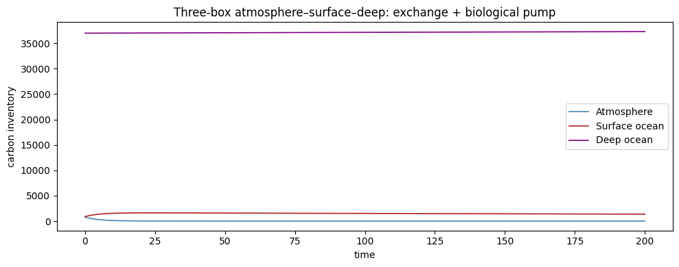

Figure. Three-box atmosphere–surface–deep system. During the pulse (\(t < 30\)) atmospheric carbon spikes and surface ocean rises slightly via air-sea exchange. After the pulse, the atmosphere relaxes quickly back toward equilibrium with the surface. The deep ocean responds on the longest timescale — the biological pump slowly transfers surface carbon downward, and by \(t=200\) has absorbed most of the perturbation.

Solver notes

RK45 is appropriate for all box models here; none are stiff under typical parameters.

TwoBoxCarbon and GenericBoxModel both use uses_post_history=True. Diagnostics (net_flux) are computed by replaying tendency callables over the solved history.

Time-varying source terms in the generic framework use register_source + a forcing registered on the corresponding 'source__<box>' parameter:

spec.register_source('A', value=0.0)
model.register_forcing('source__A', cc.Forcing(lambda t: ...))

Common pitfall: register_exchange('A', 'S', ...) and register_exchange('S', 'A', ...) would double-count the same reciprocal pathway. Always register each exchange pair once.