Noise in Models — Three Injection Modes

Author

Jordan Landers

Published

June 12, 2026

Abstract

Three independent ways to introduce stochasticity differ fundamentally in where noise enters the dynamics. Noisy forcing feeds randomness through the model’s input; SDE integration (Euler-Maruyama, Heun-Maruyama, Milstein) injects it directly into the state update; post-integration noise simulates observation error without any dynamical feedback. This notebook compares all three approaches on EBM0D.

Keywords

noise, noisy forcing, SDE, Euler-Maruyama, Heun-Maruyama, Milstein, stochastic integration, observation noise, ensemble, EBM0D

import numpy as np
import matplotlib.pyplot as plt
import climatecritters as cc
from climatecritters.model_critters.ebm import EBM0D
from climatecritters.utils import noise as cc_noise
import pyleoclim as pyleo

T_SPAN = (0, 500)   # years

Clean baseline

Run once; reuse throughout for comparison.

model_clean = EBM0D()
out_clean   = model_clean.integrate(t_span=T_SPAN, y0=[255.0], method='RK45')
T_clean     = out_clean.state_variables['T']
t_clean     = out_clean.time

Noisy forcing

Wrap a stochastic process in a cc.Forcing callable and attach it with register_forcing. The noise is part of the input, not the state equations, so the model stays deterministic and the perturbation is inspectable.

Here: AR(1) noise added to S0 (the solar constant).

Always visualise the forcing before attaching it.

t_eval = np.arange(T_SPAN[0], T_SPAN[1] + 1, dtype=float)

# AR(1): σ=3 W m⁻², τ=20 yr
sigma_drive, tau_drive = 3.0, 20.0
rng_f = np.random.default_rng(0)
noise_vals = np.zeros(len(t_eval))
for i in range(1, len(noise_vals)):
    alpha = np.exp(-1.0 / tau_drive)
    noise_vals[i] = (alpha * noise_vals[i-1]
                     + sigma_drive * np.sqrt(1 - alpha**2) * rng_f.standard_normal())

solar_noise = cc.Forcing(
    lambda t, _t=t_eval, _v=noise_vals: float(np.interp(t, _t, _v))
)

# Visualise first
fig, ax = plt.subplots(figsize=(10, 3))
ax.plot(t_eval, noise_vals, color='teal', lw=0.9)
ax.axhline(0, color='k', lw=0.7, ls=':')
ax.set_xlabel('time (yr)'); ax.set_ylabel('ΔS₀ (W m⁻²)')
ax.set_title('AR(1) solar noise forcing  (σ=3 W m⁻², τ=20 yr)')
plt.tight_layout(); plt.show()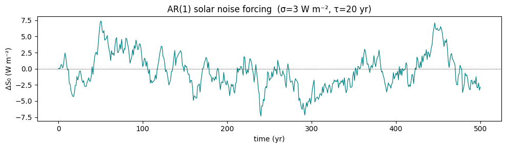

model_noisy_f = EBM0D()
model_noisy_f.register_forcing('S0', solar_noise, 'additive')
out_noisy_f   = model_noisy_f.integrate(t_span=T_SPAN, y0=[255.0], method='RK45')

fig, axes = plt.subplots(2, 1, figsize=(10, 6), sharex=True)
axes[0].plot(t_eval, noise_vals, color='teal', lw=0.9)
axes[0].axhline(0, color='k', lw=0.7, ls=':')
axes[0].set_ylabel('ΔS₀ (W m⁻²)')

axes[1].plot(t_clean, T_clean, color='gray', lw=1.5, label='clean')
axes[1].plot(out_noisy_f.time, out_noisy_f.state_variables['T'],
             color='teal', lw=1.0, alpha=0.85, label='noisy forcing')
axes[1].set_xlabel('time (yr)'); axes[1].set_ylabel('T (K)'); axes[1].legend()
axes[1].set_ylim((285,290))
fig.suptitle('EBM0D — noisy forcing vs clean')
plt.tight_layout(); plt.show()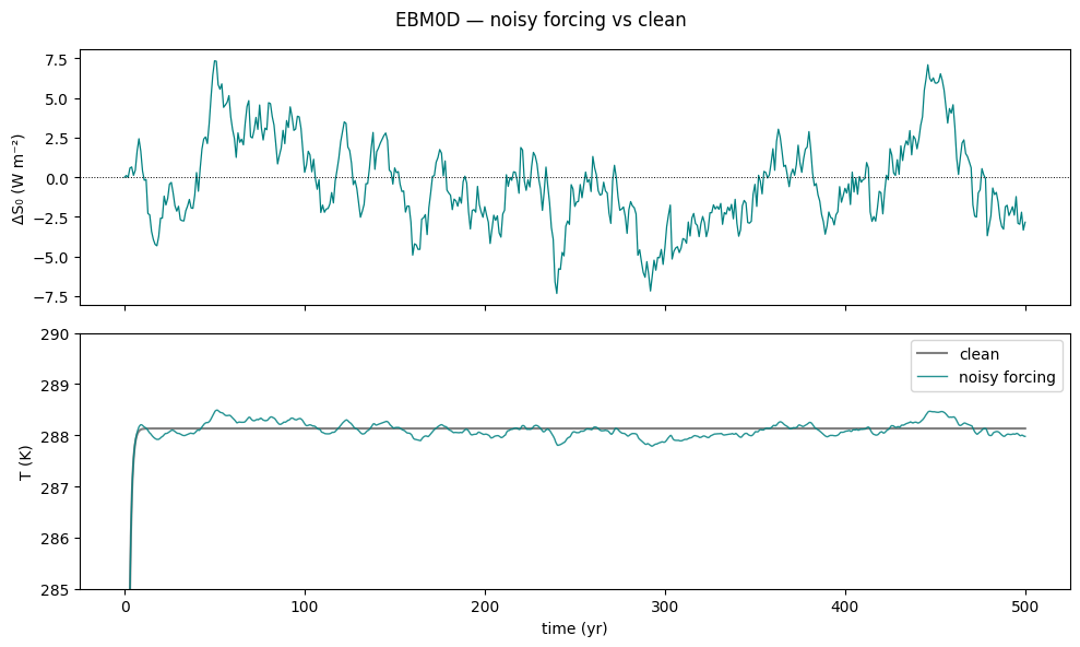

Figure. The noisy run tracks the forcing with a lag set by the thermal inertia. The perturbations never drive the model to a new equilibrium because the noise is zero-mean and the heat capacity keeps the system well-damped.

Noise during integration

SDE integrators inject noise at every timestep: \(dT = f(T)\,dt + \sigma\,dW\).

To use them: 1. Set model.sde_noise = lambda t, state: noise_scale_vector 2. Call integrate(..., method='euler_maruyama') — or heun_maruyama (strong order 1.0) or milstein (strong order 1.0, multiplicative noise) 3. Pass kwargs={'dt': ..., 'random_seed': N} — dt is required

heun_maruyama is the default recommendation: better accuracy than euler_maruyama at the same dt, with no extra cost for additive noise.

SIGMA_SDE = 0.8   # K yr⁻⁰·⁵
DT_SDE    = 0.5   # yr

def sde_noise_fn(t, state):
    return np.full_like(np.asarray(state, dtype=float), SIGMA_SDE)

# Deterministic Euler baseline vs three SDE methods
configs = [
    ('euler',         {},                          'gray',      '-',  'Euler (deterministic)'),
    ('euler_maruyama',{'random_seed': 0},          'steelblue', '-',  'Euler-Maruyama'),
    ('heun_maruyama', {'random_seed': 0},          'seagreen',  '-',  'Heun-Maruyama'),
    ('milstein',      {'random_seed': 0},          'firebrick', '--', 'Milstein'),
]

runs_sde = {}
for method, extra_kw, color, ls, label in configs:
    m = EBM0D()
    if method != 'euler':
        m.sde_noise = sde_noise_fn
    out = m.integrate(t_span=T_SPAN, y0=[255.0], method=method,
                      kwargs={'dt': DT_SDE, **extra_kw})
    runs_sde[label] = (out, color, ls)

fig, ax = plt.subplots(figsize=(10, 4))
for label, (out, color, ls) in runs_sde.items():
    lw = 1.8 if label == 'Euler (deterministic)' else 1.0
    ax.plot(out.time, out.state_variables['T'],
            color=color, ls=ls, lw=lw, alpha=0.85, label=label)
ax.set_xlabel('time (yr)'); ax.set_ylabel('T (K)')
ax.set_title(f'SDE integration  (σ={SIGMA_SDE}, dt={DT_SDE} yr)')
ax.legend(); plt.tight_layout(); plt.show()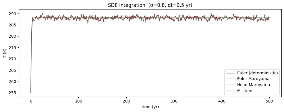

Figure. For additive noise (σ independent of state) Milstein’s correction term is zero, so Heun-Maruyama and Milstein give identical trajectories at the same seed. All three converge to the same neighbourhood of ~288 K — noise is zero-mean, so it doesn’t shift the attractor.

# Run an ensemble to characterise spread
N_ENS = 20
ens_T, ens_t = [], None
for seed in range(N_ENS):
    m = EBM0D(); m.sde_noise = sde_noise_fn
    out = m.integrate(t_span=T_SPAN, y0=[255.0], method='heun_maruyama',
                      kwargs={'dt': DT_SDE, 'random_seed': seed})
    ens_T.append(out.state_variables['T'])
    if ens_t is None:
        ens_t = out.time          # time axis from the SDE runs
ens_arr = np.array(ens_T)

# Trim the clean reference to the same length if needed
T_clean_ref = T_clean[:len(ens_t)] if len(T_clean) > len(ens_t) else T_clean
t_clean_ref = t_clean[:len(ens_t)] if len(t_clean) > len(ens_t) else t_clean

fig, ax = plt.subplots(figsize=(10, 4))
for row in ens_arr:
    ax.plot(ens_t, row, color='steelblue', lw=0.5, alpha=0.3)
ax.plot(ens_t, ens_arr.mean(axis=0), color='navy', lw=2, label='ensemble mean')
ax.plot(t_clean_ref, T_clean_ref, color='gray', lw=1.5, ls='--', label='deterministic')
ax.set_xlabel('time (yr)'); ax.set_ylabel('T (K)')
ax.set_title(f'Heun-Maruyama ensemble  ({N_ENS} realisations)')
ax.legend(); plt.tight_layout(); plt.show()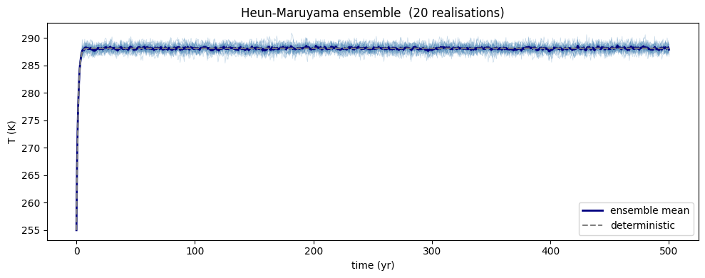

Figure. Ensemble mean converges to the deterministic equilibrium; spread is largest during the fast transient when the gradient is steepest.

Noise post-integration

Run the model cleanly, then add noise to the output series with climatecritters.utils.noise. Use this when the noise represents observation error or proxy noise rather than intrinsic variability — the dynamics stay deterministic and reproducible.

ts_clean = pyleo.Series(time=t_clean, value=T_clean,
                        time_name='time', time_unit='yr',
                        value_name='T', value_unit='K', label='deterministic')

# RK45 produces irregular timesteps — interpolate to regular grid before
# generating surrogates (ar1sim requires evenly-spaced time)
ts_clean_reg = ts_clean.interp()
t_reg = ts_clean_reg.time
T_reg = ts_clean_reg.value

# AR(1) surrogates matched to the signal's autocorrelation
surr_ar1 = cc_noise.from_series(ts_clean_reg, method='ar1sim', number=5, seed=1)

# Pink noise (β=1) from parameters
surr_cn = cc_noise.from_param(method='CN', noise_param=[1], length=len(t_reg),
                               time_pattern='specified',
                               settings={'time': t_reg}, number=5, seed=2)

fig, axes = plt.subplots(1, 2, figsize=(13, 4), sharey=True)
for ax, surr, color, title in [
        (axes[0], surr_ar1, 'steelblue', 'AR(1) observation noise'),
        (axes[1], surr_cn,  'firebrick', 'Coloured noise (β=1)'),
]:
    ax.plot(t_reg, T_reg, color='gray', lw=2, label='deterministic', zorder=3)
    for s in surr.series_list:
        noisy = T_reg + 0.5 * (s.value - s.value.mean()) / s.value.std()
        ax.plot(t_reg, noisy, color=color, lw=0.7, alpha=0.45)
    ax.set_xlabel('time (yr)'); ax.set_title(title)
axes[0].set_ylabel('T (K)')
fig.suptitle('EBM0D — post-integration noise  (5 realisations each)')
plt.tight_layout()

Time axis values sorted in ascending order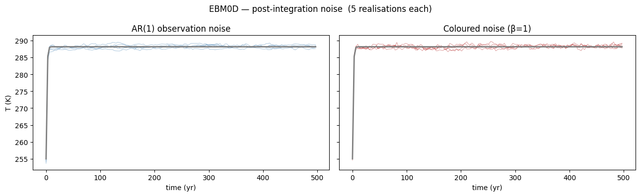

{'label': 'deterministic'}
{'label': 'deterministic'}
{'label': 'Power-law surrogates ($S(f) \\propto f^{-\\beta}$) #5'}

Figure. Both panels converge to exactly the same deterministic equilibrium — post-integration noise does not feed back into dynamics. AR(1) produces slower meanders; pink noise adds spectral richness across all scales.

Which approach to use?

	Noisy forcing	Noise during integration	Noise post-integration
Feeds back into dynamics	✓ (through input)	✓ (on state)	✗
Deterministic model preserved	✓	✗	✓
Physical interpretation	Boundary/external forcing	Intrinsic variability	Measurement / proxy noise
Reproducibility	Pre-draw + wrap	`random_seed` kwarg	`seed` in `from_series`/`from_param`
Requires SDE integrator	✗	✓	✗