Lorenz96 — Lorenz (1996) Atmospheric Model

Author

Jordan Landers

Published

June 12, 2026

Abstract

Lorenz96 implements the periodic-ring atmospheric model of Lorenz (1996) with quadratic advection and constant external forcing. This notebook covers single-scale chaotic dynamics — wave packets, westward propagation — and the two-scale extension coupling slow large-scale variables X to fast small-scale variables Y, the canonical benchmark system for data assimilation research.

Keywords

Lorenz96, atmospheric model, periodic ring, wave packets, chaos, single-scale, two-scale, fast-slow coupling, timescale separation, data assimilation

Overview

Lorenz96 implements the periodic-ring atmospheric model of Lorenz (1996), with an optional fast-variable layer from Lorenz & Emanuel (1998). Three physical processes are encoded: quadratic advection, linear damping, and external forcing.

Single-scale (`J=0`)

\[\frac{dX_i}{dt} = (X_{i+1} - X_{i-2})\,X_{i-1} - X_i + F, \qquad i = 0,\ldots,n-1\]

All indices cyclic mod \(n\). For \(F \gtrsim 5\) and \(n = 40\) the system is chaotic; the canonical value is \(F = 8\).

Two-scale (`J>0`)

Each slow variable \(X_k\) is coupled to \(J\) fast variables \(Y_{k,j}\):

\[\frac{dX_k}{dt} = (X_{k+1} - X_{k-2})\,X_{k-1} - X_k + F - \frac{hc}{b}\sum_{j=0}^{J-1} Y_{k,j}\]

\[\frac{dY_{k,j}}{dt} = -cb\,Y_{k,j+1}(Y_{k,j+2} - Y_{k,j-1}) - c\,Y_{k,j} + \frac{hc}{b}\,X_k\]

The parameter \(c\) sets the timescale ratio: \(Y\) evolves \(c\) times faster than \(X\).

Parameters

Name	Description	Default
`n`	Number of slow-scale variables	40
`J`	Fast variables per slow variable; `J=0` = single-scale	0
`F`	External forcing amplitude	8.0
`h`	Coupling coefficient X↔︎Y (two-scale only)	1.0
`b`	Y/X amplitude ratio (two-scale only)	10.0
`c`	Y/X timescale ratio (two-scale only)	10.0

F accepts a float, callable (t) / (t, state), or cc.Forcing.

import numpy as np
import matplotlib.pyplot as plt
import climatecritters as cc
from climatecritters.model_critters.lorenz import Lorenz96

rng = np.random.default_rng(42)   # fixed seed for reproducibility

Single-Scale System

The single-scale system (J=0) is the simpler starting point. Random initial conditions on \([-1, 1]\) reach the chaotic attractor within a few time units. The canonical diagnostic is the space-time diagram: colour = \(X_i\), rows = variable index, columns = time. Diagonal bands reveal westward-propagating wave packets.

n, F_canon = 40, 8.0
y0_ss = rng.uniform(-1, 1, n)

model_ss = Lorenz96(n=n, F=F_canon)
output_ss = model_ss.integrate(t_span=(0, 30), y0=y0_ss.tolist(),
                                method='rk4', dt=0.05)

t_ss = np.asarray(output_ss.time)
X_ss = np.column_stack([output_ss.state_variables[f'x{i}'] for i in range(n)])
print(f"X shape: {X_ss.shape}  ({X_ss.shape[0]} time steps \u00d7 {n} variables)")

X shape: (601, 40)  (601 time steps × 40 variables)

fig, ax = plt.subplots(figsize=(10, 5))
im = ax.imshow(
    X_ss.T, aspect='auto', origin='lower',
    extent=[t_ss[0], t_ss[-1], -0.5, n - 0.5],
    cmap='RdBu_r', vmin=-10, vmax=10,
)
plt.colorbar(im, ax=ax, label='$X_i$')
ax.set_xlabel('time'); ax.set_ylabel('variable index $i$')
ax.set_title(f'Single-scale Lorenz-96 — space-time diagram  (n={n}, F={F_canon})')
plt.tight_layout(); plt.show()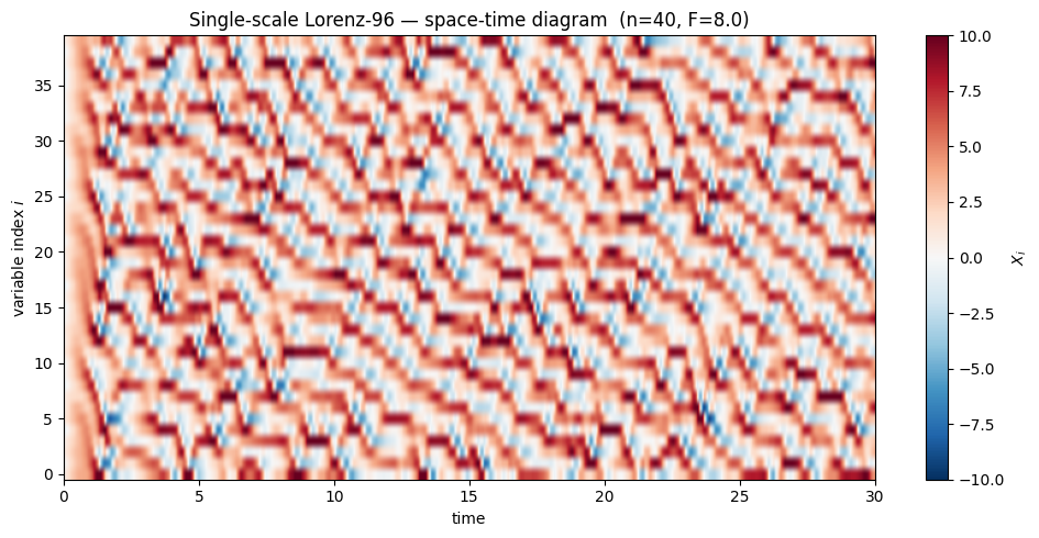

Reading the space-time diagram. Each row is one of the \(n=40\) model variables arranged around a ring; each column is a snapshot in time. Warm colours (red) indicate positive anomalies; cool (blue) indicate negative. The diagonal stripes are wave packets travelling around the ring: the tilt from lower-left to upper-right means each packet moves toward higher variable indices as time advances. Packets grow, break, and reform continuously — the hallmark of deterministic chaos. No two rows are in phase for long; coherence is lost within roughly one Lyapunov time (\(\approx 0.6\)–\(1\) time units for \(F=8\)), which sets the limit of predictability.

The variables \(X_i\) are sometimes interpreted as anomalies of some atmospheric quantity (e.g. vorticity or temperature) at equally spaced longitudes on a mid-latitude circle. The “westward” propagation of wave packets then corresponds to Rossby-wave-like behaviour — though Lorenz96 is a toy model and should not be over-interpreted physically.

The `F` parameter

F is the external forcing amplitude. Low F (≲ 5) gives ordered, low-amplitude wave structures; high F gives fully developed chaos with larger excursions and shorter predictability. Below, F=4 (weakly chaotic) is compared with F=8 (canonical) using the same initial condition:

F_vals = [4.0, 8.0]

# gridspec: two equal plot columns + a narrow dedicated colorbar column
fig = plt.figure(figsize=(13, 4))
gs  = fig.add_gridspec(1, 3, width_ratios=[1, 1, 0.05], wspace=0.12)
ax0 = fig.add_subplot(gs[0, 0])
ax1 = fig.add_subplot(gs[0, 1], sharey=ax0)
cax = fig.add_subplot(gs[0, 2])

for ax, F_val in zip([ax0, ax1], F_vals):
    m = Lorenz96(n=n, F=F_val)
    out = m.integrate(t_span=(0, 30), y0=y0_ss.tolist(),
                      method='rk4', dt=0.05)
    t = np.asarray(out.time)
    X = np.column_stack([out.state_variables[f'x{i}'] for i in range(n)])
    im = ax.imshow(X.T, aspect='auto', origin='lower',
                   extent=[t[0], t[-1], -0.5, n - 0.5],
                   cmap='RdBu_r', vmin=-10, vmax=10)
    ax.set_xlabel('time'); ax.set_title(f'F = {F_val}')

ax0.set_ylabel('variable index $i$')
ax1.tick_params(labelleft=False)
fig.colorbar(im, cax=cax, label='$X_i$')
fig.suptitle('Single-scale Lorenz-96 — effect of forcing amplitude F')
plt.show()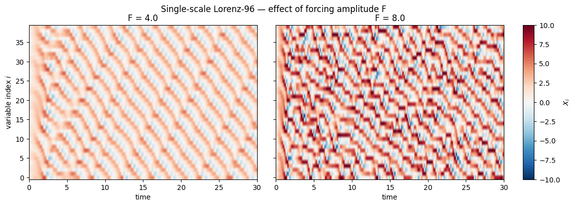

What changes with \(F\). At \(F=4\) the waves are longer-lived: coherent stripes stretch across several time units before breaking, and the amplitude range is smaller (shading stays within roughly \(\pm 5\)). At \(F=8\) the stripes break up much faster, excursions are larger (shading reaches \(\pm 10\)), and consecutive snapshots at the same \(i\) look nearly uncorrelated after one or two time units. This compression of the predictability horizon is the practical meaning of “stronger forcing = more chaos” in this model. For \(F \lesssim 5\) the system is only weakly chaotic or even periodic; the canonical \(F=8\) sits well inside the fully turbulent regime.

Two-Scale System

Setting J > 0 activates the coupled fast-variable layer. Each slow variable \(X_k\) drives \(J\) fast variables \(Y_{k,j}\), which feed back on \(X_k\) through the coupling sink. With the default \(c = 10\), \(Y\) evolves ten times faster than \(X\).

The fast variables require a warmup. Random initial conditions place the system far from the two-scale attractor; a short integration (≈ 10 time units) discards the transient before diagnostics are taken.

Solver requirement: use method='rk4' with a small fixed timestep dt and a coarser recording interval si (passed via kwargs). Adaptive solvers (RK45) call dydt at unpredictable sub-steps that corrupt the accumulated state for this model.

K, J_val = 36, 10
F_ts = 10.0

# IC: slow vars near the forcing level, fast vars near zero
y0_ts = np.concatenate([rng.standard_normal(K) + F_ts,
                         rng.standard_normal(K * J_val) * 0.01])

# --- warmup: reach the two-scale attractor ---
model_warm = Lorenz96(n=K, J=J_val, F=F_ts)
warmup = model_warm.integrate(t_span=(0, 10), y0=y0_ts.tolist(),
                               method='rk4', dt=0.005,
                               kwargs={'si': 0.05})

# Extract the final state as the production IC
y0_warm = np.array(
    [warmup.state_variables[f'x{k}'][-1] for k in range(K)] +
    [warmup.state_variables[f'y{j}'][-1] for j in range(K * J_val)]
)

# --- production run: si=0.005 resolves Y dynamics (timescale ~ 1/c = 0.1) ---
model_ts = Lorenz96(n=K, J=J_val, F=F_ts)
output_ts = model_ts.integrate(t_span=(0, 20), y0=y0_warm.tolist(),
                                method='rk4', dt=0.005,
                                kwargs={'si': 0.005})

t_ts = np.asarray(output_ts.time)
X_ts = np.column_stack([output_ts.state_variables[f'x{k}'] for k in range(K)])
Y_ts = np.column_stack([output_ts.state_variables[f'y{j}'] for j in range(K * J_val)])
print(f"X shape: {X_ts.shape}  (slow)")
print(f"Y shape: {Y_ts.shape}  (fast)")

X shape: (4001, 36)  (slow)
Y shape: (4001, 360)  (fast)

# Zoom to first 5 time units to make individual Y oscillations visible
mask = t_ts <= 5.0
Y_block0 = Y_ts[:, :J_val]   # Y_{0,j} for j = 0..J-1

fig, axes = plt.subplots(2, 1, figsize=(11, 5), sharex=True)

axes[0].plot(t_ts[mask], X_ts[mask, 0], lw=1.2, color='steelblue')
axes[0].set_ylabel('$X_0$ (slow)')
axes[0].set_title(f'Two-scale Lorenz-96 — timescale separation  (K={K}, J={J_val}, c=10)')

# J fast variables attached to X_0; each oscillates ~10x faster than X
for j in range(J_val):
    axes[1].plot(t_ts[mask], Y_block0[mask, j], lw=0.5, alpha=0.7)
axes[1].set_ylabel('$Y_{0,j}$ (fast)')
axes[1].set_xlabel('time')

plt.tight_layout(); plt.show()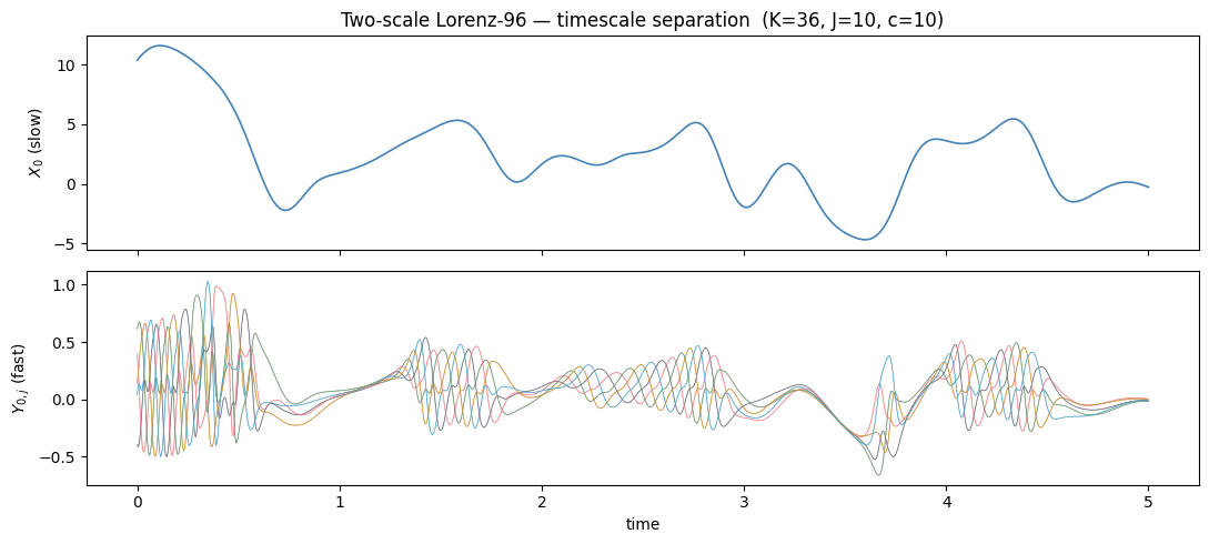

What the two panels show. The upper panel (\(X_0\)) is the slow “resolved” variable — it evolves on order-1 time units and looks like a typical L96 trajectory. The lower panel shows the \(J=10\) fast variables \(Y_{0,j}\) attached to \(X_0\). They oscillate roughly \(c=10\) times faster than \(X_0\) and with amplitudes scaled by \(1/b = 0.1\) relative to the slow scale. Their net effect on \(X_0\) enters as the coupling sink \(-\frac{hc}{b}\sum_j Y_{0,j}\), which acts like a stochastic sub-grid drag — reducing the effective forcing seen by the slow variables.

The two-scale system is the standard benchmark for data assimilation and parameterisation research: the \(X\) variables represent the “truth” that a model must track, while the \(Y\) variables represent unresolved processes that a coarser model would need to parameterise.

fig, axes = plt.subplots(1, 2, figsize=(13, 5))

im0 = axes[0].imshow(
    X_ts.T, aspect='auto', origin='lower',
    extent=[t_ts[0], t_ts[-1], -0.5, K - 0.5],
    cmap='RdBu_r',
)
plt.colorbar(im0, ax=axes[0], label='$X_k$')
axes[0].set_xlabel('time'); axes[0].set_ylabel('$k$')
axes[0].set_title('Slow variables $X_k(t)$')

im1 = axes[1].imshow(
    Y_ts.T, aspect='auto', origin='lower',
    extent=[t_ts[0], t_ts[-1], -0.5, K * J_val - 0.5],
    cmap='RdBu_r',
)
plt.colorbar(im1, ax=axes[1], label='$Y_{k,j}$')
axes[1].set_xlabel('time'); axes[1].set_ylabel('$k \\cdot J + j$')
axes[1].set_title('Fast variables $Y_{k,j}(t)$')

fig.suptitle(f'Two-scale Lorenz-96 — space-time  (K={K}, J={J_val}, F={F_ts})')
plt.tight_layout(); plt.show()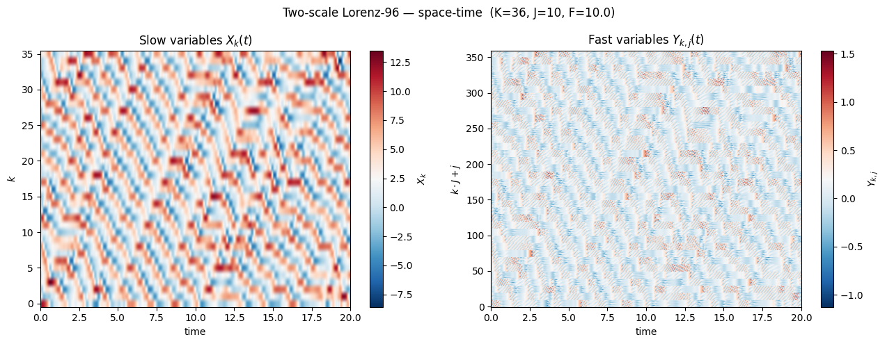

Comparing the two space-time diagrams. The left panel (\(X_k\)) looks qualitatively like the single-scale diagram — propagating wave packets on the slow timescale. The right panel (\(Y_{k,j}\)) has \(K \times J = 360\) rows. They are ordered as \(Y_{0,0},\ldots,Y_{0,J-1},\,Y_{1,0},\ldots\) so every \(J=10\) rows corresponds to a new host variable \(X_k\); the repeating block structure is visible as horizontal banding every 10 rows. Within each block the \(J\) fast variables share the same slow-scale envelope (inherited from \(X_k\)) but carry rapid fine-scale oscillations. The Y field consequently looks like a “textured” version of X: the large-scale wave pattern is still faintly visible, but the dominant visual impression is rapid, small-scale variability.

Solver notes

Single-scale (J=0): RK45 (adaptive) or rk4 (fixed step) both work. dt=0.05 is adequate for space-time diagnostics at \(F=8\).

Two-scale (J>0): always use method='rk4' with explicit dt and si. Adaptive solvers call dydt at sub-step evaluations that corrupt the accumulated state history for this model.

output = model.integrate(t_span=..., y0=..., method='rk4',
                         dt=0.005, kwargs={'si': 0.005})

dt: integration timestep — keep ≤ 0.005 for the two-scale system to resolve fast-variable dynamics
si: recording interval — set equal to dt to capture all Y oscillations, or larger to downsample

Accessing Y for variable k: output.state_variables[f'y{k*J + j}'] for \(j = 0,\ldots,J-1\).

Warmup is required for the two-scale system. Random initial conditions placed far from the attractor take ≈ 5–10 time units to equilibrate. Always discard a warmup run before taking statistics or diagnostics.