Forcing — Time-Varying Inputs

Author

Jordan Landers

Published

June 12, 2026

Abstract

cc.Forcing is the unified interface for all time-varying inputs in ClimateCritters. This notebook covers every construction pattern — callable functions, array+time pairs, composable Hold/Ramp/Harmonic elements, and bundled CSV datasets — along with attachment options, timing control, and guidance on using forcing with SDE solvers.

Keywords

Forcing, Hold, Ramp, Harmonic, register_forcing, attachment_style, timing, callable, interpolation, SDE

import numpy as np
import matplotlib.pyplot as plt
import climatecritters as cc

Construction patterns

1. Callable

Any function of time t. No pre-processing, no interpolation overhead. The simplest way to express analytical signals.

# Any Python callable works — constant, polynomial, sinusoidal, etc.
f_const  = cc.Forcing(lambda t: 1.0)
f_linear = cc.Forcing(lambda t: 0.01 * t)
f_sin    = cc.Forcing(lambda t: np.sin(2 * np.pi * t / 10.0))

fig, axes = plt.subplots(1, 3, figsize=(12, 3))
for ax, f, label in zip(axes,
                        [f_const, f_linear, f_sin],
                        ["constant", "linear", "sinusoidal"]):
    f.plot(t_span=(0, 50), ax=ax)
    ax.set_title(label); ax.set_xlabel("time")
plt.suptitle("Callable forcings", y=1.02)
plt.tight_layout(); plt.show()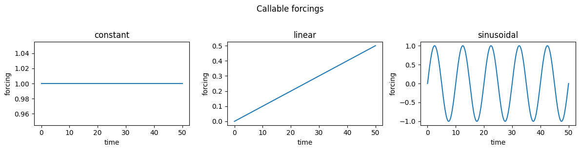

2. Array + time axis

Interpolated from a data array and a matching time axis. Default interpolation is cubic spline; pass interpolation="linear" for piecewise linear. Useful for wrapping proxy records, reanalysis output, or any pre-computed time series.

# Sparse data record (e.g. a proxy reconstruction at irregular time points)t_data = np.array([  0., 10., 20., 30., 40., 50.])v_data = np.array([  0.,  1.,  0.5, 2.,  1.,  0.])f_cubic  = cc.Forcing(data=v_data, time=t_data,                      plot_kwargs={'color': 'steelblue', 'label': 'cubic spline'})f_linear = cc.Forcing(data=v_data, time=t_data, interpolation="linear",                      plot_kwargs={'color': 'firebrick', 'linestyle': '--', 'label': 'linear interp'})

fig, ax = plt.subplots(figsize=(8, 3))ax.scatter(t_data, v_data, color="k", zorder=3, label="data points")f_cubic.plot(ax=ax)f_linear.plot(ax=ax)ax.set_xlabel("time"); ax.legend()ax.set_title("Array forcing — cubic vs linear interpolation")plt.tight_layout(); plt.show()

3. `from_sequence` — composable elements

Three element types chain end-to-end in time. Each element’s start value is inferred from the previous element’s end value when not specified explicitly.

The elements are: Ramp (monotonic transition), Harmonic (sinusoidal), and Hold (constant connector between other elements).

Components

`Ramp` — monotonic transition

Ramp(duration, y0, yf, shape) transitions between two values over duration time units. shape is "linear" (default) or "cosine" (smooth S-curve, no discontinuous derivative at the endpoints).

r_linear = cc.forcing.Ramp(duration=10, y0=0.0, yf=3.0, shape="linear")
r_cosine = cc.forcing.Ramp(duration=10, y0=0.0, yf=3.0, shape="cosine")

fig, ax = plt.subplots(figsize=(7, 3))
r_linear.plot(ax=ax, label="linear")
r_cosine.plot(ax=ax, linestyle="--", label="cosine")
ax.set_xlabel("time"); ax.set_title("Ramp shapes: linear vs cosine easing")
ax.legend(); plt.tight_layout(); plt.show()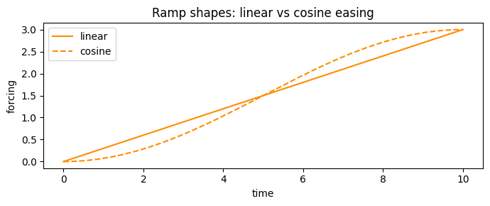

`Harmonic` — sinusoidal segment

Harmonic(duration, period, A, center) generates a sinusoidal signal for duration time units. The phase is set automatically so the segment starts at the value inherited from the previous element (or at center if it is the first).

harm = cc.forcing.Harmonic(duration=50, period=10, A=1.5, center=0.0)

fig, ax = harm.plot()
ax.set_xlabel("time"); ax.set_title("Harmonic element (period=10, A=1.5)")
plt.tight_layout(); plt.show()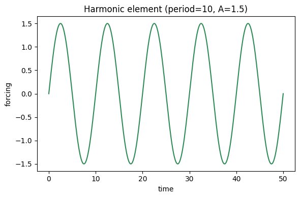

`Hold` — constant segment

Hold(duration, value) holds a constant value for duration time units. Most useful as a connector — a baseline before a perturbation, or a plateau after a ramp.

Building a sequence

from_sequence accepts a list of elements. Here a solar dimming-recovery scenario: two holds and two ramps (one linear, one cosine for variety), surrounding a period of reduced solar output. Each piece is shown individually first, then the full signal with segments colored by element type.

# Define each piece — colors set at construction via plot_kwargs
piece1 = cc.forcing.Hold(duration=100, value=1365.0,                             plot_kwargs={'color': 'steelblue'})   # baseline hold
piece2 = cc.forcing.Ramp(duration=50,  y0=1365.0, yf=1300.0, shape="cosine",    plot_kwargs={'color': 'firebrick'})   # cosine ramp down
piece3 = cc.forcing.Hold(duration=100, value=1300.0,                             plot_kwargs={'color': 'coral'})       # hold at reduced S0
piece4 = cc.forcing.Ramp(duration=50,  y0=1300.0, yf=1365.0, shape="linear",    plot_kwargs={'color': 'seagreen'})    # linear ramp back up
piece5 = cc.forcing.Hold(duration=200, value=1365.0,                             plot_kwargs={'color': 'steelblue'})   # return to baseline

# Keep as ForcingSequence so .plot() can colour segments by element type
solar_seq = piece1 + piece2 + piece3 + piece4 + piece5

# Individual pieces in their own subplots — default element colors apply
pieces = [piece1, piece2, piece3, piece4, piece5]
labels = ["Hold\n1365", "Cosine ramp\n↓ to 1300", "Hold\n1300",
          "Linear ramp\n↑ to 1365", "Hold\n1365"]

fig, axes = plt.subplots(1, 5, figsize=(14, 3))
for i, (piece, label) in enumerate(zip(pieces, labels)):
    piece.plot(ax=axes[i])
    axes[i].set_title(label, fontsize=8)
    axes[i].set_ylim(1285, 1380)
    axes[i].set_xlabel("time (within piece)")
    if i == 0:
        axes[i].set_ylabel("S₀ (W m⁻²)")

plt.suptitle("Individual pieces", y=1.02)
plt.tight_layout(); plt.show()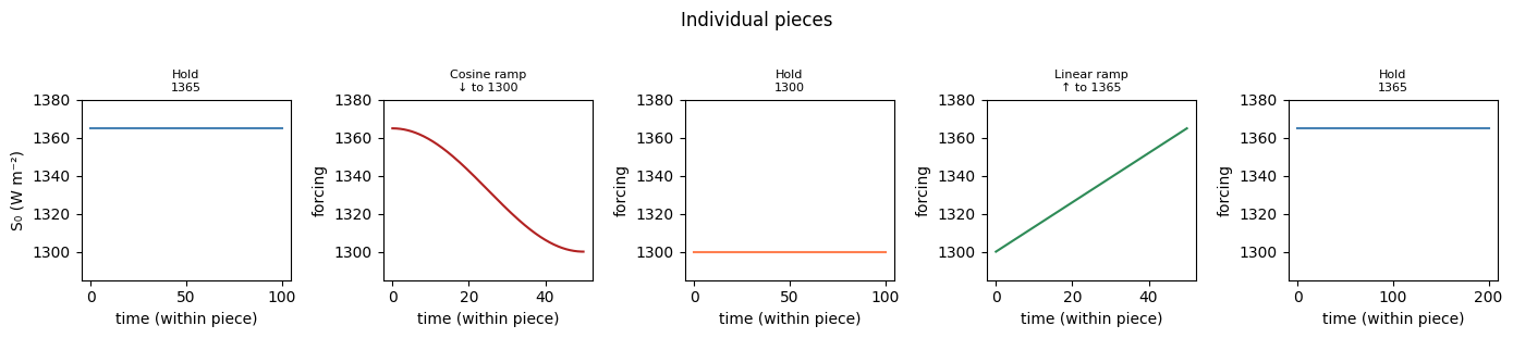

# Full sequence — segments coloured by element type automatically
fig, ax = solar_seq.plot()
ax.set_xlabel("time"); ax.set_ylabel("S₀ (W m⁻²)")
ax.set_title("Composed solar_seq — segments coloured by element type")
plt.tight_layout(); plt.show()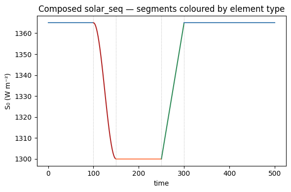

Composing with `+`

Elements can be chained with + instead of building a list — returns a ForcingSequence that Forcing() accepts directly. Equivalent to from_sequence, just more readable for short sequences.

f_seq = (
    cc.forcing.Hold(duration=100, value=1365.0)
    + cc.forcing.Ramp(duration=50,  y0=1365.0, yf=1300.0, shape="cosine")
    + cc.forcing.Hold(duration=350, value=1300.0)
)

fig, ax = f_seq.plot()
ax.set_xlabel("time"); ax.set_ylabel("S₀ (W m⁻²)")
ax.set_title("Composed with + operator")
plt.tight_layout(); plt.show()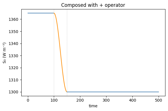

4. `from_csv` — bundled datasets

Two datasets are bundled with ClimateCritters:

tsi   = cc.Forcing.from_csv(dataset="vieira_tsi")   # Total Solar Irradiance, yr BP
insol = cc.Forcing.from_csv(dataset="insolation")   # 65°N insolation anomaly, kyr

print(f"vieira_tsi:  t = {tsi.time.min():.0f} – {tsi.time.max():.0f} yr BP, "
      f"S0 = {tsi.data.min():.2f} – {tsi.data.max():.2f} W m⁻²")
print(f"insolation:  t = {insol.time.min():.0f} – {insol.time.max():.0f} kyr, "
      f"range = {insol.data.min():.1f} – {insol.data.max():.1f}")

vieira_tsi:  t = 0 – 7840 yr BP, S0 = 340.01 – 340.41 W m⁻²
insolation:  t = -5000 – 0 kyr, range = -61.6 – 70.8

fig, axes = plt.subplots(2, 1, figsize=(10, 5))

tsi.plot(ax=axes[0], color="goldenrod", lw=0.8)
axes[0].invert_xaxis()
axes[0].set_xlabel("yr BP"); axes[0].set_ylabel("TSI (W m⁻²)")
axes[0].set_title("Vieira et al. total solar irradiance reconstruction")

insol.plot(ax=axes[1], color="steelblue", lw=0.8)
axes[1].set_xlabel("kyr"); axes[1].set_ylabel("insolation anomaly")
axes[1].set_title("Orbital insolation at 65°N")

plt.tight_layout(); plt.show()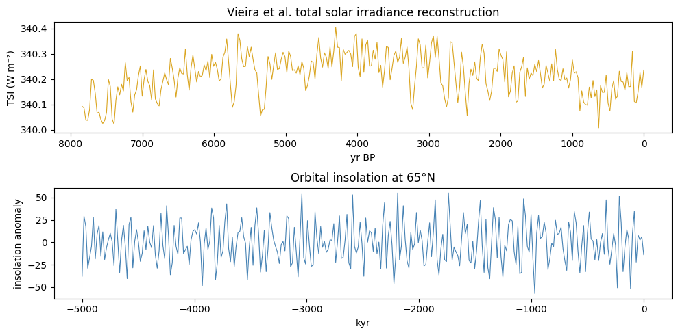

`register_forcing` — attaching to a model

register_forcing(var_name, forcing_obj, attachment_style, timing) wires a Forcing object into a model’s integration loop. It wraps dydt transparently — no changes to the model subclass are needed.

There are two target types (parameter or state variable) and two dimensions of control (attachment style and timing):

Attachment style: `"replacement"` vs `"additive"`

"replacement" — the forcing value substitutes the current parameter or state completely. Nothing else is added; the original value is irrelevant during that step.

"additive" — the forcing value is injected on top of whatever the model is already computing. For a parameter this is the natural way to add centred noise: k = k₀ + ε(t). For a state variable it acts as an external source or sink term added to dxdt (pre) or x (post).

Timing: “pre” vs “post”

"pre" — applied inside the right-hand side at each solver function evaluation. For a parameter replacement, param_values is temporarily patched so get_param_value sees the forced value throughout dydt. For an additive state variable, the forcing value is added to dxdt[idx] — it enters as a rate (same units as dx/dt).

"post" — applied after each accepted integration step. For state replacement, x[idx] is set to forcing(t) — prescribing the state directly (useful for nudging or data assimilation). For additive state, forcing(t) is added to x[idx] as a finite jump per step.

Adaptive solvers and post-step: "post" timing requires a fixed-step solver ("euler", "rk4", "euler_maruyama"). Adaptive solvers ("RK45" and other scipy.integrate.solve_ivp methods) do not expose a per-step callback, so post-step forcings are silently skipped — CCModel.integrate() will emit a warning.

Valid combinations by target

Target	Style	Timing	Effect
Parameter	`replacement`	`pre` (only option)	`param_values[name]` is patched to `forcing(t)` during each `dydt` call
Parameter	`additive`	`pre` (only option)	`forcing(t)` is added to the nominal parameter value: `param_values[name] + forcing(t)`
State var	`replacement`	`post` (only option)	`x[idx]` is set to `forcing(t)` after each accepted step (fixed-step solvers only)
State var	`additive`	`pre`	`forcing(t)` is added to `dxdt[idx]` — a continuous source/sink rate
State var	`additive`	`post`	`forcing(t)` is added to `x[idx]` after each step (fixed-step only)

# Parameter replacement — time-varying solar constant
model.register_forcing("S0", cc.Forcing(lambda t: 1365.0 + 5*np.sin(t)))

# Parameter additive — white noise on a diffusion coefficient
rng = np.random.default_rng(42)
model.register_forcing("D", cc.Forcing(lambda t: rng.normal(0, 0.01)),
                       attachment_style="additive")

# State additive pre — freshwater flux into salinity tendency
model.register_forcing("S", cc.Forcing(lambda t: 0.1),
                       attachment_style="additive", timing="pre")

Inspecting and clearing

model.get_forcings()            # dict of all registered forcings
model.get_forcings("S0")        # list of ForcingSpec for one variable
model.clear_forcings()          # remove all forcings
model.clear_forcings("S0")      # remove forcings on one variable only

Noise and stochastic forcing

Noise can enter a model through register_forcing or through dedicated SDE solvers:

Via register_forcing — wrap any stochastic callable in a Forcing and attach it as an additive state variable forcing. This is convenient for post-hoc exploration but mixes noise into the deterministic solver, which can affect step-size selection in adaptive solvers.

rng = np.random.default_rng(42)
noise = cc.Forcing(lambda t: rng.normal(0, 0.05))   # white noise
model.register_forcing("S", noise, "additive", timing="pre")

Via SDE solvers — the cleanest approach for stochastic integration. Define sde_noise(t, x) on the model and pass a stochastic method to integrate():

# heun_maruyama: strong order 1 for additive noise
output = model.integrate(t_span=(0, 100), y0=[...], method="heun_maruyama",
                         dt=0.1, random_seed=42)
# milstein: strong order 1 for multiplicative noise (diffusion depends on state)
output = model.integrate(t_span=(0, 100), y0=[...], method="milstein",
                         dt=0.1, random_seed=42)

See the noise utilities (cc.utils.noise) for post-hoc noise application to already-integrated output.

Construction patterns

1. Callable

2. Array + time axis

3. from_sequence — composable elements

Components

Ramp — monotonic transition

Harmonic — sinusoidal segment

Hold — constant segment