core.forcing.Ramp

core.forcing.Ramp(
    duration=None,
    y0=None,
    yf=None,
    A=None,
    y_exit=None,
    shape='linear',
    plot_kwargs=None,
)

Monotonic transition between two values with linear or cosine easing.

Parameters

duration : float = None: Length of the transition.
y0 : float = None: Starting value. If omitted, inherits from the previous segment’s endpoint.
yf : float = None: Ending value. If omitted, computed from A or y_exit.
A : float = None: Signed amplitude of the transition (yf = y0 + A). Used when yf is not specified directly.
y_exit : float = None: Absolute target value combined with A and duration to compute a proportionally scaled duration.
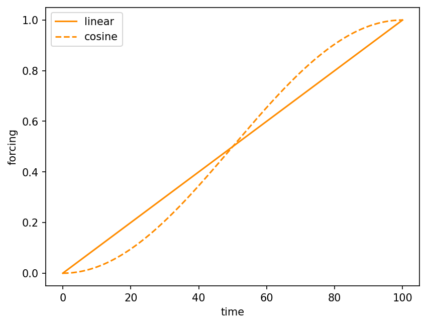
shape : ('linear', 'cosine') = 'linear': Interpolation shape. 'cosine' gives a smooth S-curve (eased start and end); 'linear' is a straight line. Default 'linear'.

Notes

The shape='cosine' option applies a half-cosine ease, producing an S-curve::

y(τ) = y0 + (yf - y0) * 0.5 * (1 - cos(π * τ / duration))

This is smoother than 'linear' at both endpoints and is a good choice when the transition is intended to represent a gradual forcing change rather than an abrupt one.

Examples

import matplotlib.pyplot as plt
import climatecritters as cc

fig, ax = plt.subplots()
cc.forcing.Ramp(100, y0=0.0, yf=1.0, shape='linear').plot(ax=ax, label='linear')
cc.forcing.Ramp(100, y0=0.0, yf=1.0, shape='cosine').plot(ax=ax, label='cosine', linestyle='--')
ax.legend()
plt.savefig('docs/reference/figures/Ramp_shapes_example.png',
            dpi=150, bbox_inches='tight')