Model3

Model3(
    var_name='ice volume',
    f1=-16,
    f2=16,
    t1=30,
    t2=10,
    vc=1.4,
    insolation=0.0,
    state_variables=['v', 'k'],
    non_integrated_state_vars=['k'],
    diagnostic_variables=['insolation'],
    *args,
    **kwargs,
)

Model 3 from Ganopolski (2024) describing glacial cycle evolution under orbital forcing.

The model tracks ice volume v and glacial regime k (1 = glaciation, 2 = deglaciation). The ice volume relaxes toward a forcing-dependent equilibrium:

dv/dt = (ve(f) - v) / t1    when k=1  (glaciation)
dv/dt = -vc / t2             when k=2  (deglaciation)

Regime switches follow:

k=1 → k=2 if v > vc, df/dt > 0, and f > 0
k=2 → k=1 if f < f1

Parameters

var_name : str = 'ice volume': Label for the model output. Default 'ice volume'.
f1 : float or callable or cc.Forcing = -16: Insolation threshold for glacial inception (W/m^2; typically -20 to -15). Default -16.
f2 : float or callable or cc.Forcing = 16: Insolation threshold for deglaciation inception (W/m^2; typically positive). Default 16.
t1 : float or callable or cc.Forcing = 30: Relaxation timescale for glacial inception (kyr). Default 30.
t2 : float or callable or cc.Forcing = 10: Relaxation timescale for deglaciation (kyr). Default 10.
vc : float or callable or cc.Forcing = 1.4: Critical ice volume controlling dominant periodicity and asymmetry. Default 1.4.

Notes

State variables are v (ice volume, normalised) and k (regime index, non-integrated). The diagnostic variable insolation records f(t) at each output step.

The insolation parameter (default 0.0) provides the orbital forcing value used by the model. Register a time-varying orbital signal via::

model.register_forcing('insolation', cc.Forcing(calc_f))

The internal derivative of forcing dfdt is computed via :func:calc_df by default; supply a custom callable or cc.Forcing to override.

Parameter defaults are taken from Ganopolski (2024). Time-varying parameters follow the standard callable contract (t), (t, state), or (t, state, model).

References

Ganopolski, A. (2024). Glacial cycles. Nature Reviews Earth & Environment, 5, 89–106.

Examples

import climatecritters as cc
from climatecritters.model_critters.g24 import Model3, calc_f
import matplotlib.pyplot as plt

model = Model3()
model.register_forcing('insolation', cc.Forcing(calc_f))

output = model.integrate(
    t_span=(-2000, 0), y0=[0.0, 1], method='RK45',
    kwargs={'max_step': 0.5}
)
ts = output.to_pyleo(var_names=['v'])
ts.plot()
plt.savefig('docs/reference/figures/Model3_example.png',
            dpi=150, bbox_inches='tight')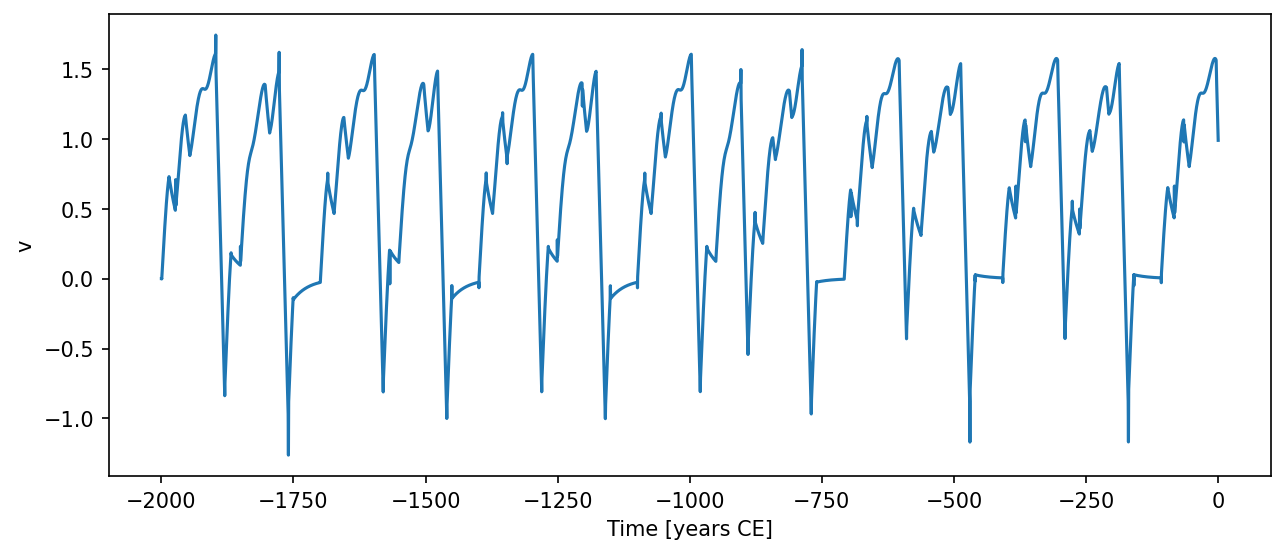

Methods

Name	Description
calc_dfdt	Evaluate df/dt — the time derivative of the orbital forcing at time `t`.
calc_vc	Evaluate the critical ice volume `vc` (constant or time/state-varying).
calc_ve	Equilibrium ice volume toward which the system is attracted.
calc_vg	Glacial equilibrium ice volume.
calc_vu	Unstable equilibrium ice volume separating glacial and interglacial basins.
dydt	Evaluate ice-volume tendency at time `t` and state `x`.

calc_dfdt

Model3.calc_dfdt(t, x=None)

Evaluate df/dt — the time derivative of the orbital forcing at time t.

calc_vc

Model3.calc_vc(t, x=None)

Evaluate the critical ice volume vc (constant or time/state-varying).

calc_ve

Model3.calc_ve(v, f, f1, f2, vi=0)

Equilibrium ice volume toward which the system is attracted.

In the bi-stable regime (f1 < f < f2) the target depends on the current ice volume v relative to the unstable equilibrium vu.

Parameters

v : float: Current ice volume (normalised).
f : float: Orbital forcing value (W/m^2).
f1 : float: Lower insolation threshold (glaciation onset).
f2 : float: Upper insolation threshold (deglaciation onset).
vi : float = 0: Interglacial equilibrium ice volume. Default 0.

Returns

ve : float: Target equilibrium ice volume.

calc_vg

Model3.calc_vg(f, f1, f2)

Glacial equilibrium ice volume.

Parameters

f : float: Orbital forcing value (W/m^2).
f1 : float: Lower insolation threshold.
f2 : float: Upper insolation threshold.

Returns

vg : float: Glacial equilibrium ice volume.

calc_vu

Model3.calc_vu(f, f1, f2)

Unstable equilibrium ice volume separating glacial and interglacial basins.

Parameters

f : float: Orbital forcing value (W/m^2).
f1 : float: Lower insolation threshold.
f2 : float: Upper insolation threshold.

Returns

vu : float: Unstable equilibrium ice volume.

dydt

Model3.dydt(t, x)

Evaluate ice-volume tendency at time t and state x.

Returns

: list of float: [dvdt] — the ice-volume tendency. The regime index k is a non-integrated state variable updated in-place.