Lorenz96
Lorenz96(
    var_name='lorenz96',
    n=40,
    J=0,
    F=8.0,
    h=1.0,
    b=10.0,
    c=10.0,
    exact_rhs=False,
    state_variables=None,
    diagnostic_variables=None,
    *args,
    **kwargs,
)
Lorenz (1996) single-scale and two-scale atmospheric model.
A periodic ring of n slow-scale variables with quadratic advection and constant forcing:
dX_k/dt = (X_{k+1} - X_{k-2}) * X_{k-1} - X_k + FWhen J > 0 a second, faster Y layer of n × J variables is coupled to the slow layer (the two-scale system of Lorenz & Emanuel 1998):
dX_k/dt = ... - (h*c/b) * sum_j Y_{j,k}
dY_{j,k}/dt = -c*b * Y_{j+1,k} * (Y_{j+2,k} - Y_{j-1,k}) - c*Y_{j,k} + (h*c/b)*X_k
Parameters
var_name : str = 'lorenz96'-
Label for the model output. Default
'lorenz96'. n : int = 40-
Number of slow-scale variables. Default 40.
J : int = 0-
Fast variables per slow variable.
J=0(default) gives the single-scale system;J>0activates the two-scale system. F : float or callable orcc.Forcing= 8.0-
Slow-scale forcing amplitude. Default 8.0. Pass a time-varying signal via
model.register_forcing('F', forcing_obj). h : float = 1.0-
Coupling coefficient between X and Y layers (two-scale only). Default 1.0.
b : float = 10.0-
Amplitude ratio Y/X (two-scale only). Default 10.0.
c : float = 10.0-
Timescale ratio Y/X (two-scale only). Default 10.0.
exact_rhs : bool = False-
If
True, use globalnp.rollon the flattened Y vector, matching the original L96_model.py reference implementation. DefaultFalse(per-block loop, identical results).
Notes
For the two-scale system (J>0) use method='rk4' with a small fixed time step passed directly to integrate::
output = model.integrate(t_span=..., y0=..., method='rk4',
                         dt=0.005, kwargs={'si': 0.05})
Adaptive solvers (RK45) call dydt at unpredictable sub-steps; the fixed-step RK4 avoids this problem. Plain Euler is too coarse to resolve the fast Y dynamics.
References
Lorenz, E. N. (1996). Predictability: A problem partly solved. Lorenz, E. N., & Emanuel, K. A. (1998). J. Atmos. Sci., 55, 399–414.
Examples
import matplotlib.pyplot as plt
import numpy as np
import climatecritters as cc
from climatecritters.model_critters.lorenz import Lorenz96
# Single-scale system
model = Lorenz96(n=40, F=8.0)
y0 = np.random.randn(40) + 8.0
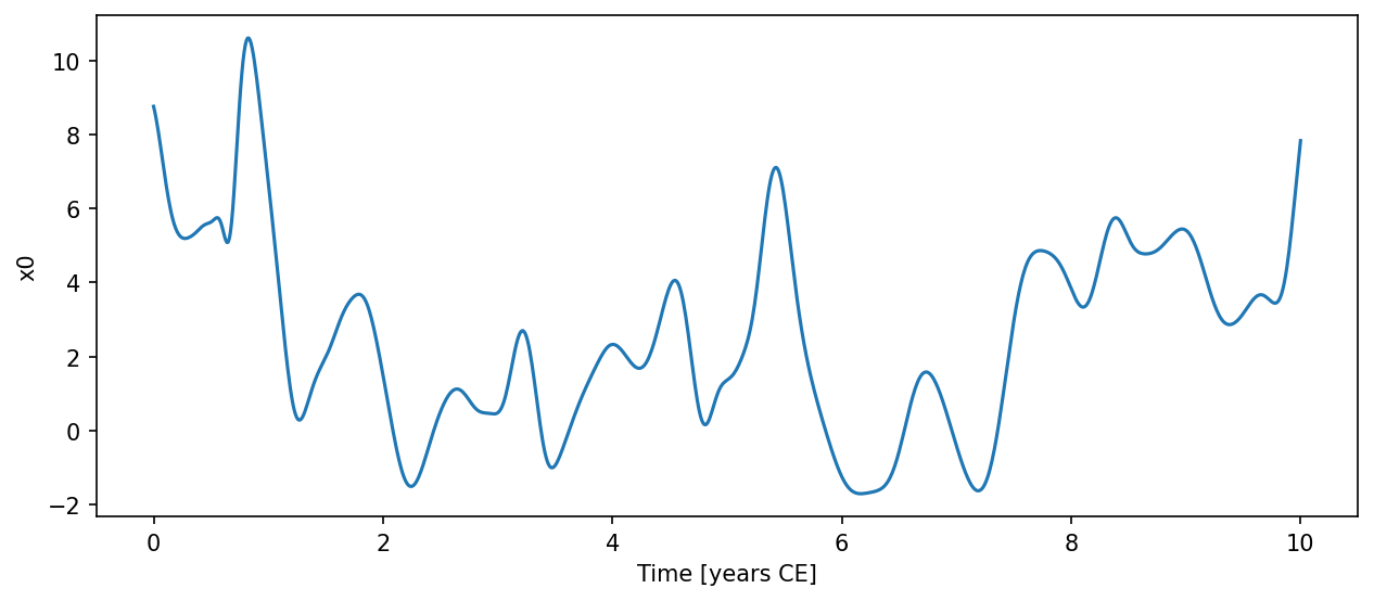
output = model.integrate(t_span=(0, 10), y0=y0, method='rk4', dt=0.01)
ts = output.to_pyleo(var_names=['x0'])
# Two-scale system
K, J = 36, 10
model2 = Lorenz96(n=K, J=J, F=10.0)
y0_2 = np.concatenate([np.random.randn(K) + 10.0,
np.random.randn(K * J) * 0.01])
output2 = model2.integrate(t_span=(0, 10), y0=y0_2,
method='rk4', dt=0.005,
kwargs={'si': 0.05})
ts = output.to_pyleo(var_names=['x0'])
ts.plot()
plt.savefig('docs/reference/figures/Lorenz96_example.png',
dpi=150, bbox_inches='tight')