Stocker2003BipolarSeesaw

Stocker2003BipolarSeesaw(
    var_name='stocker2003_bipolar_seesaw',
    tau=1000.0,
    beta=-1.0,
    Tn=0.0,
    state_variables=None,
    diagnostic_variables=None,
    *args,
    **kwargs,
)

Minimum thermodynamic model for the thermal bipolar seesaw.

A single prognostic southern temperature anomaly Ts relaxes toward a northern temperature signal Tn(t) scaled by beta:

dTs/dt = (beta*Tn(t) - Ts) / tau

Parameters

var_name : str = 'stocker2003_bipolar_seesaw': Label for the model output. Default 'stocker2003_bipolar_seesaw'.
tau : float or callable or cc.Forcing = 1000.0: Thermal equilibration timescale (years). Must be > 0. Default 1000.
beta : float or callable or cc.Forcing = -1.0: Amplitude ratio relating southern to northern anomaly. Default -1.0 (antiphase seesaw).
Tn : float or callable or cc.Forcing = 0.0: Northern temperature anomaly. Default 0.0. Register a time-varying signal via model.register_forcing('Tn', forcing_obj).

Notes

The diagnostic variable Tn (northern temperature) is written by populate_diagnostics_from_history after integration. State variable is Ts.

References

Stocker, T. F., & Johnsen, S. J. (2003). A minimum thermodynamic model for the bipolar seesaw. Paleoceanography, 18(4), 1087.

Examples

import numpy as np
import climatecritters as cc
from climatecritters.model_critters.stocker2003_bipolar_seesaw import (
    Stocker2003BipolarSeesaw,
)

import matplotlib.pyplot as plt

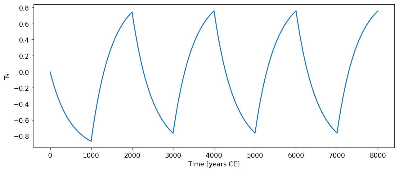
model = Stocker2003BipolarSeesaw(tau=500.0, beta=-1.0)
model.register_forcing('Tn', cc.Forcing(lambda t: 1.0 if (t % 2000) < 1000 else -1.0))
output = model.integrate(
    t_span=(0, 8000), y0=[0.0], method='RK45'
)
ts = output.to_pyleo(var_names=['Ts'])
ts.plot()
plt.savefig('docs/reference/figures/Stocker2003BipolarSeesaw_example.png',
            dpi=150, bbox_inches='tight')