TwoBoxCarbon

TwoBoxCarbon(
    var_name='two_box_carbon',
    k=0.2,
    R=0.0,
    l_s=0.0,
    V_atm=1.0,
    V_surf=1.0,
    state_variables=None,
    diagnostic_variables=None,
    *args,
    **kwargs,
)

Two-box carbon exchange model with explicit box volumes.

State variables A and S are carbon inventories (mass units) in the atmospheric and surface-ocean boxes respectively. Air-sea exchange is driven by the concentration gradient:

exchange = k * (A/V_atm - S/V_surf)
dA/dt = -exchange + R - l_s*A
dS/dt = exchange

Parameters

var_name : str = 'two_box_carbon': Label for the model output. Default 'two_box_carbon'.
k : float or callable or cc.Forcing = 0.2: Air-sea gas exchange rate constant (volume units per time). Default 0.2.
R : float or callable or cc.Forcing = 0.0: Constant carbon source flux into the atmosphere (mass per time). Default 0.0. Register a time-varying source via model.register_forcing('R', forcing_obj).
l_s : float or callable or cc.Forcing = 0.0: First-order atmospheric loss coefficient. Default 0.0.
V_atm : float or callable or cc.Forcing = 1.0: Volume of the atmospheric box (must be > 0). Default 1.0.
V_surf : float or callable or cc.Forcing = 1.0: Volume of the surface-ocean box (must be > 0). Default 1.0.

Notes

Diagnostic variable net_flux (the atmospheric tendency dA/dt) is computed in populate_diagnostics_from_history after integration.

V_atm and V_surf must be positive; ValueError is raised if either is ≤ 0.

Examples

import climatecritters as cc
from climatecritters.model_critters.two_box_carbon import TwoBoxCarbon
import matplotlib.pyplot as plt

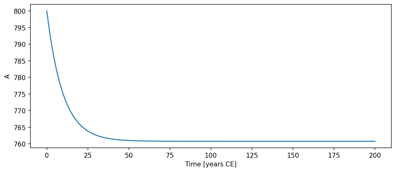
model = TwoBoxCarbon(k=0.1, V_atm=1.0, V_surf=50.0)
output = model.integrate(
    t_span=(0, 200), y0=[800.0, 38000.0], method='RK45'
)
ts = output.to_pyleo(var_names=['A'])
ts.plot()
plt.savefig('docs/reference/figures/TwoBoxCarbon_example.png',
            dpi=150, bbox_inches='tight')