EBM0D

EBM0D(
    var_name='temperature',
    state_variables=None,
    diagnostic_variables=None,
    OLR=None,
    C=4,
    albedo=0.3,
    S0=1365.0,
)

Zero-dimensional energy balance model for global-mean surface temperature.

Evolves global-mean surface temperature T according to:

C dT/dt = (1 - alpha) * S0/4 - OLR

where S0 is the solar constant, alpha is the planetary albedo, and OLR is the outgoing longwave radiation.

Parameters

state_variables : list of str = None

Names of the integrated state variables. Default is ['T'].

diagnostic_variables : list of str = None

Names of diagnostic quantities accumulated during integration. Default is ['albedo', 'absorbed_SW', 'OLR', 'solar_incoming'].

var_name : str = 'temperature'

Label for the modeled quantity. Default is 'temperature'.

OLR : callable or None = None

Outgoing longwave radiation. Must have a compliant signature: (t), (t, state), or (t, state, model) with the first argument named t or time (see contracts/signal_model_contract.md). Default is Stefan-Boltzmann via OLR_func(pRad=650, ps=1000).

C : float or callable or cc.Forcing = 4

Heat capacity (W yr m⁻² K⁻¹). If callable, must follow the parameter callable contract. Default is 4.

albedo : float or callable or cc.Forcing = 0.3

Planetary albedo. If callable, must follow the parameter callable contract. Default is 0.3.

S0 : float or callable or cc.Forcing = 1365.0

Solar constant (W m⁻²). Default 1365.0. Pass a time-varying orbital signal via model.register_forcing('S0', forcing_obj).

Notes

State variable is T (global-mean surface temperature, K). Diagnostic variables albedo, absorbed_SW, OLR, and solar_incoming are accumulated step-by-step during integration.

All parameters support time-varying callables or Forcing objects; they are resolved at each timestep via get_param_value.

See also

EBM1DLat : Latitudinally-resolved 1D variant. OLR_func : Default OLR callable factory. albedo_func : Ice-albedo callable for use as the albedo parameter.

Examples

import matplotlib.pyplot as plt
import climatecritters as cc
from climatecritters.model_critters.ebm import EBM0D

model = EBM0D(S0=1360.0)
output = model.integrate(t_span=(0, 500), y0=[288.0], method='RK45')
ts = output.to_pyleo(var_names=['T'])
ts.plot()
plt.savefig('docs/reference/figures/EBM0D_example.png',
            dpi=150, bbox_inches='tight')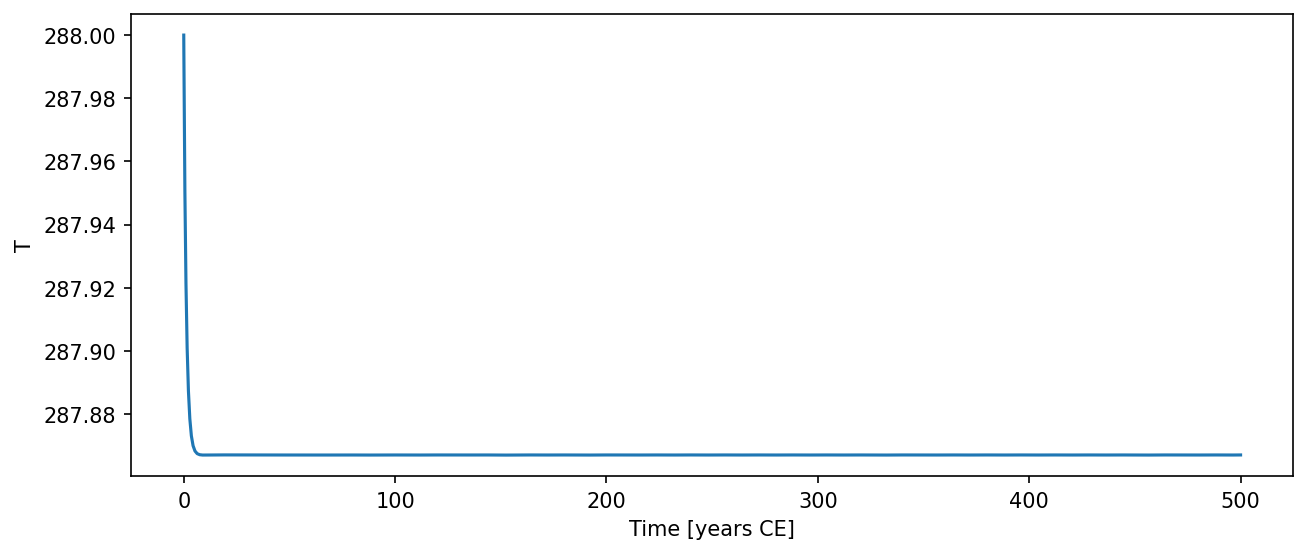

EBM0D example output

With a time-varying albedo and custom OLR:

from climatecritters.model_critters.ebm import EBM0D, albedo_func, OLR_func

model = EBM0D(albedo=albedo_func, OLR=OLR_func(pRad=600))

Methods

Name	Description
dydt	Evaluate the right-hand side of the ODE at time t and state x.

dydt

EBM0D.dydt(t, x)

Evaluate the right-hand side of the ODE at time t and state x.

Called by the solver at each timestep. As a side effect, appends the current state to self.state_variables and appends each diagnostic quantity to the corresponding list in self.diagnostic_variables.

Parameters

t : float

Current time.

x : array - like

Current state vector. x[0] is the global-mean temperature T (K).

Returns

dydt : list of float

Time-derivatives [dT/dt].