core.Forcing

core.Forcing(
    data,
    time=None,
    params=None,
    interpolation='cubic',
    plot_kwargs=None,
)

Unified time-varying signal consumed by models.

Forcing wraps any time-dependent input and exposes a single get_forcing(t) interface to the model.

Input types

Pass a callable, a data array, a bundled CSV dataset, or a compiled ForcingSequence::

# callable
f = cc.Forcing(lambda t: 1360.0 + 5.0 * np.sin(2 * np.pi * t / 11.0))

# data array
f = cc.Forcing(data=values, time=t_axis, interpolation='cubic')

# bundled CSV dataset
f = cc.Forcing.from_csv(dataset='vieira_tsi')
f = cc.Forcing.from_csv(file_path='my_data.csv', time_name='age', value_name='co2')

# ForcingSequence (auto-compiled)
seq = cc.forcing.Hold(100, value=0.0) + cc.forcing.Ramp(50, y0=0.0, yf=4.0)
f   = cc.Forcing(seq)

Value superposition

Two Forcing objects (or a Forcing and a callable) can be combined with + to produce a new Forcing whose value is the pointwise sum::

combined = cc.Forcing(orbital_func) + cc.Forcing(noise_func)

A bounded ForcingElement or ForcingSequence can also be superposed; it is auto-compiled and the result is bounded to that element’s duration.

Full operator table:

Left	Right	Result	Semantic
Forcing	Forcing	Forcing (indefinite)	value superposition for all t
Forcing	callable	Forcing (indefinite)	value superposition for all t
ForcingElement	ForcingElement	ForcingSequence	temporal concatenation
ForcingSequence	ForcingElement / ForcingSequence	ForcingSequence	temporal concatenation
ForcingElement / ForcingSequence	Forcing	Forcing (bounded)	additive overlay; auto-compiles
Forcing	ForcingElement / ForcingSequence	Forcing (bounded)	additive overlay; auto-compiles

Parameters

data : callable, array-like, or ForcingSequence

The signal source. See Input types above.

time : array - like = None

Time axis for array-backed Forcing. Must be strictly increasing and the same length as data. If omitted, integer indices are used.

params : dict = None

Extra keyword arguments forwarded to a callable data via functools.partial.

interpolation : ('cubic', 'linear') = 'cubic'

Interpolation method for array-backed Forcing. Default 'cubic'.

plot_kwargs : dict = None

Matplotlib keyword arguments used by .plot() — e.g. color, linewidth, label, linestyle. Explicit kwargs passed to .plot() override these defaults.

Examples

import matplotlib.pyplot as plt
import climatecritters as cc

scenario = (
    cc.forcing.Hold(200, value=280.0)
    + cc.forcing.Ramp(100, y0=280.0, yf=560.0, shape='cosine')
    + cc.forcing.Hold(200, value=560.0)
)
fig, ax = scenario.compile().plot()
plt.savefig('docs/reference/figures/Forcing_sequence_example.png',
            dpi=150, bbox_inches='tight')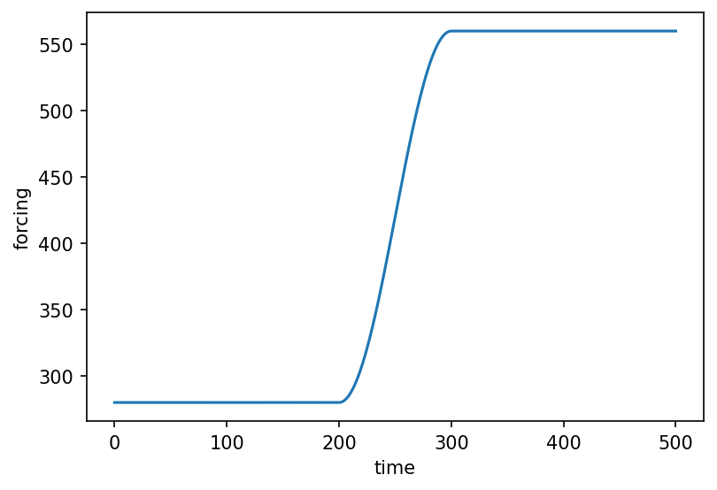

Forcing_sequence example output

Methods

Name	Description
from_csv	Build a Forcing from a CSV file or a bundled dataset.
from_sequence	Build a Forcing from an iterable of ForcingElement parts.
get_forcing	Return the forcing value at time t.
plot	Plot the forcing signal over a time range.

from_csv

core.Forcing.from_csv(
    dataset=None,
    file_path=None,
    value_name=None,
    time_name=None,
    params=None,
    interpolation='cubic',
)

Build a Forcing from a CSV file or a bundled dataset.

Two datasets are included with ClimateCritters:

• 'vieira_tsi' — Vieira et al. total solar irradiance reconstruction
• 'insolation' — 65°N summer solstice insolation (Laskar et al.)

Parameters

dataset : ('vieira_tsi', 'insolation') = 'vieira_tsi'

Name of a bundled dataset. Mutually exclusive with file_path.

file_path : str or Path = None

Path to an arbitrary CSV file. Mutually exclusive with dataset.

value_name : str = None

Column name for the forcing values. If omitted, the first column (or the dataset default) is used.

time_name : str = None

Column name for the time axis. If omitted, integer indices are used (or the dataset default is applied).

params : dict = None

Extra keyword arguments forwarded to the interpolator.

interpolation : ('cubic', 'linear') = 'cubic'

Interpolation method. Default 'cubic'.

Returns

forcing : Forcing

Examples

import climatecritters as cc

# Bundled dataset
tsi = cc.Forcing.from_csv(dataset='vieira_tsi')

# Custom CSV
co2 = cc.Forcing.from_csv(
    file_path='data/co2_record.csv',
    time_name='age_kyr',
    value_name='co2_ppm',
    interpolation='linear',
)

from_sequence

core.Forcing.from_sequence(parts, label='forcing')

Build a Forcing from an iterable of ForcingElement parts.

Convenience alias for ForcingSequence(parts, label).compile().

Parameters

parts : iterable of ForcingElement

Ordered Hold, Ramp, Harmonic, or general ForcingElement instances defining the piecewise timeline.

label : str = 'forcing'

Human-readable label for the resulting forcing object.

Returns

forcing : Forcing

Examples

import climatecritters as cc

f = cc.Forcing.from_sequence([
    cc.forcing.Hold(duration=100, value=0.0),
    cc.forcing.Ramp(duration=50, y0=0.0, yf=1.0, shape='cosine'),
    cc.forcing.Hold(duration=100, value=1.0),
], label='freshwater_hosing')

get_forcing

core.Forcing.get_forcing(t)

Return the forcing value at time t.

Parameters

t : float or array - like

Time value(s). Accepts scalars or NumPy arrays; returns the same shape.

Returns

: float or ndarray

plot

core.Forcing.plot(t_span=None, n=300, ax=None, **kwargs)

Plot the forcing signal over a time range.

Parameters

t_span : (float, float) = None

Time range (t0, tf) to evaluate and plot. For sequence-backed Forcing objects this defaults to (0, summary["t_end"]). For array-backed objects it defaults to (time[0], time[-1]). For callable-backed objects t_span is required.

n : int = 300

Number of evaluation points. Default 300.

ax : matplotlib.axes.Axes = None

Axes to plot into. A new figure is created if None.

****kwargs** : = {}

Additional keyword arguments forwarded to ax.plot (e.g. color, linewidth, label).

Returns

fig : matplotlib.figure.Figure

ax : matplotlib.axes.Axes

Raises

: ValueError

If t_span is not provided for a callable-backed Forcing that has no time axis.

Examples

import numpy as np
import matplotlib.pyplot as plt
import climatecritters as cc

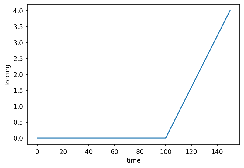
# Sequence-backed — t_span inferred automatically
f = cc.Forcing.from_sequence([
    cc.forcing.Hold(100, value=0.0),
    cc.forcing.Ramp(50, y0=0.0, yf=4.0),
])
fig, ax = f.plot()
plt.savefig('docs/reference/figures/Forcing_plot_example.png',
            dpi=150, bbox_inches='tight')

# Callable-backed — t_span required
solar = cc.Forcing(lambda t: 1360.0 + 5.0 * np.sin(t))
fig, ax = solar.plot(t_span=(0, 50))
plt.savefig('docs/reference/figures/Forcing_plot_callable_example.png',
            dpi=150, bbox_inches='tight')

Forcing_plot example output