EBM1DLat

EBM1DLat(
    var_name='ebm1d_lat',
    grid_n=50,
    C=10.0,
    D=0.55,
    A=210.0,
    B=2.0,
    S0=1365.0,
    CO2_forcing=0.0,
    state_variables=None,
    diagnostic_variables=None,
)

Diffusive annual-mean latitudinal energy balance model (Budyko-Sellers type).

Evolves the zonal-mean temperature profile T(phi) on a latitude grid:

C dT/dt = S(x)(1 - alpha(T)) - OLR(T) + D * div(grad T)

where x = sin(phi), OLR follows the Budyko linear form (A - CO2_forcing) + B * T, and diffusion is computed in x-coordinates with no-flux polar boundary conditions.

Parameters

var_name : str = 'ebm1d_lat'

Label for the modeled quantity. Default is 'ebm1d_lat'.

grid_n : int = 50

Number of evenly-spaced latitude grid points from -90° to 90°. Must be ≥ 3. Default is 50.

C : float or callable or cc.Forcing = 10.0

Heat capacity (W yr m⁻² K⁻¹). Default is 10.0.

D : float or callable or cc.Forcing = 0.55

Meridional diffusion coefficient. Default is 0.55.

A : float or callable or cc.Forcing = 210.0

Budyko OLR intercept (W m⁻²). Default is 210.0.

B : float or callable or cc.Forcing = 2.0

Budyko OLR slope (W m⁻² K⁻¹). Default is 2.0.

S0 : float or callable or cc.Forcing = 1365.0

Solar constant (W m⁻²). Default is 1365.0.

CO2_forcing : float or callable or cc.Forcing = 0.0

Radiative forcing from CO2 (W m⁻²); shifts the OLR intercept down, warming the climate. Default is 0.0.

state_variables : list of str = None

Names of the integrated state variables. Defaults to ['T_0', 'T_1', ..., 'T_{grid_n-1}'].

diagnostic_variables : list of str = None

Names of diagnostic quantities computed from the solved trajectory. Default is ['ice_line_lat', 'Tglobal'].

Notes

State variables are T_0 through T_{grid_n-1} (one temperature per latitude band, ordered from south pole to north pole). Diagnostic variables ice_line_lat and Tglobal are derived after integration.

validate_initial_state accepts a scalar and broadcasts it uniformly to the full grid.

All parameters (C, D, A, B, S0, CO2_forcing) are registered in param_values and can be swapped for callables or Forcing objects. Callables must follow the contract (t), (t, state), or (t, state, model).

See also

EBM0D : Zero-dimensional variant. EBMBase : Shared base class. albedo_func1D : Latitudinally-resolved albedo callable.

Examples

import matplotlib.pyplot as plt
import numpy as np
from climatecritters.model_critters.ebm import EBM1DLat

grid_n = 50
model = EBM1DLat(S0=1365.0, grid_n=grid_n)
output = model.integrate(
    t_span=(0, 200), y0=np.full(grid_n, 15.0), method='RK45'
)
# Plot the equilibrium latitude–temperature profile
T_final = [output.state_variables[f'T_{i}'][-1] for i in range(grid_n)]
phi = np.linspace(-90, 90, grid_n)
fig, ax = plt.subplots()
ax.plot(phi, T_final)
ax.set_xlabel('Latitude (°)'); ax.set_ylabel('Temperature (°C)')
plt.savefig('docs/reference/figures/EBM1DLat_example.png',
            dpi=150, bbox_inches='tight')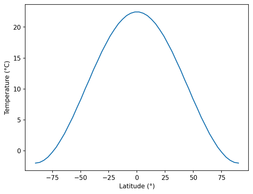

EBM1DLat example output

With a CO2 ramp:

import matplotlib.pyplot as plt
import climatecritters as cc
from climatecritters.model_critters.ebm import EBM1DLat

co2_ramp = cc.Forcing.from_sequence([
    cc.forcing.Hold(duration=100, value=0.0),
    cc.forcing.Ramp(duration=100, y0=0.0, yf=4.0, shape='linear'),
])
model_co2 = EBM1DLat(CO2_forcing=co2_ramp, D=0.35)
output_co2 = model_co2.integrate(t_span=(0, 200), y0=[15.0], method='RK45')
fig, ax = plt.subplots()
ax.plot(output_co2.time, output_co2.diagnostic_variables['Tglobal'])
ax.set_xlabel('time'); ax.set_ylabel('T_global (°C)')
ax.set_title('EBM1DLat — CO₂ ramp forcing')
plt.savefig('docs/reference/figures/EBM1DLat_co2_example.png',
            dpi=150, bbox_inches='tight')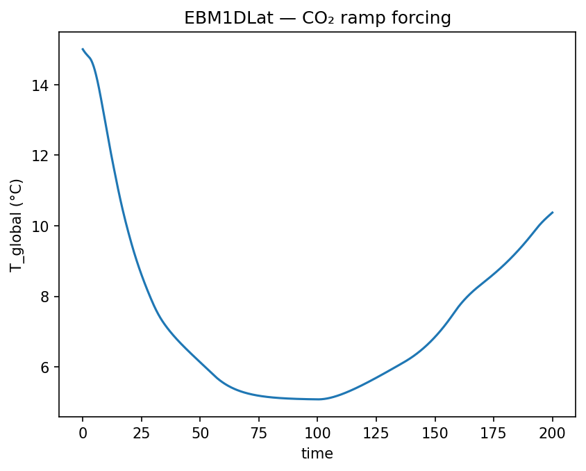

EBM1DLat_co2 example output

Methods

Name	Description
annual_mean_insolation	Compute annual-mean insolation with a P2 latitudinal distribution.
calc_OLR	Compute the Budyko linear OLR: (A - CO2_forcing) + B * T.
calc_albedo	Compute the latitudinal ice-albedo with a linear transition zone.
calc_diffusion	Compute meridional heat diffusion in x = sin(phi) coordinates.
calc_global_mean	Compute the cosine-weighted global mean temperature.
calc_ice_line_lat	Interpolate the ice-line latitude from the temperature profile.
dydt	Evaluate the right-hand side of the PDE at time t and state.
populate_diagnostics_from_history	Compute diagnostic variables from the full solved trajectory.
validate_initial_state	Validate and normalize the initial temperature profile.

annual_mean_insolation

EBM1DLat.annual_mean_insolation(t, state)

Compute annual-mean insolation with a P2 latitudinal distribution.

Approximates the zonal-mean annual-mean absorbed solar radiation as:

S(x) = (S0 / 4) * s(x),    s(x) = 1 - 0.482 * P2(sin phi)

where P2 is the second Legendre polynomial and x = sin(phi).

Parameters

t : float

Current time, passed to get_param_value for time-varying S0.

state : array - like

Current state vector (used only to satisfy the callable contract when resolving S0).

Returns

insolation : ndarray of float, shape (grid_n,)

Annual-mean insolation at each latitude grid point (W m⁻²).

calc_OLR

EBM1DLat.calc_OLR(T, t)

Compute the Budyko linear OLR: (A - CO2_forcing) + B * T.

Overrides :meth:EBMBase.calc_OLR. Parameters A, B, and CO2_forcing are resolved through get_param_value, so they can be time-varying or Forcing objects.

Parameters

T : (array - like, shape(grid_n))

Current temperature profile.

t : float

Current time, passed to get_param_value for time-varying params.

Returns

olr : ndarray of float, shape (grid_n,)

Outgoing longwave radiation at each latitude grid point (W m⁻²).

calc_albedo

EBM1DLat.calc_albedo(T, t)

Compute the latitudinal ice-albedo with a linear transition zone.

Overrides :meth:EBMBase.calc_albedo. Each grid point is assigned an albedo based on local temperature: 0.6 below -10 °C, 0.3 above 0 °C, and a linear blend in between.

Parameters

T : (array - like, shape(grid_n))

Current temperature profile (°C or K — the threshold values -10 and 0 assume °C; ensure consistency with initial conditions).

t : float

Current time. Unused; kept for a uniform external signature.

Returns

albedo : ndarray of float, shape (grid_n,)

Albedo at each latitude grid point, in [0.3, 0.6].

calc_diffusion

EBM1DLat.calc_diffusion(temperature, t, state)

Compute meridional heat diffusion in x = sin(phi) coordinates.

Applies no-flux boundary conditions at the poles by setting the diffusive flux to zero at the first and last grid points before taking the divergence.

Parameters

temperature : (array - like, shape(grid_n))

Current temperature profile.

t : float

Current time, passed to get_param_value for time-varying D.

state : array - like

Current full state vector (used only to satisfy the callable contract when resolving D).

Returns

diffusion : ndarray of float, shape (grid_n,)

Diffusive heat flux convergence at each grid point (W m⁻²), scaled by the transport factor pi/2.

calc_global_mean

EBM1DLat.calc_global_mean(temperature)

Compute the cosine-weighted global mean temperature.

Parameters

temperature : (array - like, shape(grid_n))

Zonal-mean temperature profile at one timestep.

Returns

Tglobal : float

Area-weighted global mean temperature in the same units as input.

calc_ice_line_lat

EBM1DLat.calc_ice_line_lat(temperature)

Interpolate the ice-line latitude from the temperature profile.

Defines the ice line as the -10 °C isotherm. Computes the ice-line latitude independently in each hemisphere using linear interpolation between the two adjacent grid points that straddle the threshold, then returns the average of the two hemispheric values.

Special cases: returns 90° if a hemisphere is entirely above the threshold (no ice) and 0° if entirely at or below it (full ice cover).

Parameters

temperature : (array - like, shape(grid_n))

Zonal-mean temperature profile at one timestep.

Returns

ice_line_lat : float

Mean hemispheric ice-line latitude in degrees from the equator (range [0°, 90°]).

dydt

EBM1DLat.dydt(t, state)

Evaluate the right-hand side of the PDE at time t and state.

Computes the net energy flux at each latitude grid point from insolation, ice-albedo feedback, Budyko OLR, and meridional diffusion.

This method has no side effects: because uses_post_history = True, all output is derived from the full solved trajectory in :meth:populate_diagnostics_from_history rather than accumulated here.

Parameters

t : float

Current time.

state : (array - like, shape(grid_n))

Current zonal-mean temperature profile.

Returns

dTdt : ndarray of float, shape (grid_n,)

Time-derivative of the temperature at each latitude grid point.

populate_diagnostics_from_history

EBM1DLat.populate_diagnostics_from_history(time, history)

Compute diagnostic variables from the full solved trajectory.

Called automatically by :meth:CCModel.post_integrate after the solver completes. Populates self.diagnostic_variables with the global-mean temperature and ice-line latitude at every timestep.

Parameters

time : (array - like, shape(n_steps))

Solver time axis.

history : (ndarray, shape(n_steps, grid_n))

Full temperature trajectory; each row is the temperature profile at one timestep.

validate_initial_state

EBM1DLat.validate_initial_state(y0)

Validate and normalize the initial temperature profile.

Overrides :meth:CCModel.validate_initial_state to accept a scalar initial condition and broadcast it uniformly across the latitude grid.

Parameters

y0 : float or array - like

Initial temperature(s). A scalar is broadcast to all grid_n grid points. An array must have length exactly grid_n.

Returns

y0_arr : ndarray of float, shape (grid_n,)

Validated and grid-length initial temperature array.