Roessler — Single-Scroll Chaotic Oscillator

Abstract

Roessler implements the Rössler (1976) three-variable strange attractor, characterized by a single scroll with simpler geometry than the Lorenz butterfly. This notebook shows the periodic-to-chaotic transition as parameter c increases through a period-doubling cascade, and illustrates how nonlinear coupling in the z-equation generates deterministic chaos from simple spiral dynamics.

Keywords

Roessler, strange attractor, single-scroll, chaos, period-doubling, bifurcation, phase portrait, nonlinear coupling, quasi-periodic, Rössler 1976

Overview

The Rössler system (1976) is a minimal three-variable ODE with a single-scroll strange attractor:

Equations

\[\frac{dx}{dt} = -y - z\] \[\frac{dy}{dt} = x + a\,y\] \[\frac{dz}{dt} = b + z(x - c)\]

Compared to Lorenz63, the attractor is simpler: one scroll rather than two. The variable z spikes periodically while x and y circulate quasi-periodically in the plane below. Chaos arises from the nonlinear \(z(x-c)\) term — when \(x > c\) the \(z\) variable grows exponentially before being reset.

Parameters

Name	Description	Default (canonical chaos)
a	y-feedback strength	0.2
b	z-equation offset	0.2
c	Nonlinear threshold	5.7

c controls the bifurcation structure: small c → periodic orbits; large c → chaos. State variables: x, y, z. No diagnostic variables.

import numpy as np
import matplotlib.pyplot as plt
from climatecritters.model_critters.roessler import Roessler

Canonical attractor

# a=0.2, b=0.2, c=5.7 — canonical chaotic parameter set
model = Roessler()
output = model.integrate(t_span=(0, 300), y0=[0.1, 0.0, 0.0], method='RK45')

x = output.state_variables['x']
y = output.state_variables['y']
z = output.state_variables['z']
t = output.time

print(f'Steps: {len(t)}')
print(f'x range: [{np.min(x):.2f}, {np.max(x):.2f}]')
print(f'z range: [{np.min(z):.2f}, {np.max(z):.2f}]')

Steps: 8029
x range: [-9.08, 11.41]
z range: [0.00, 22.60]

fig, axes = plt.subplots(1, 2, figsize=(12, 4))

# x-z projection — the characteristic single scroll
axes[0].plot(x, z, lw=0.25, color='steelblue', alpha=0.7)
axes[0].set_xlabel('x'); axes[0].set_ylabel('z')
axes[0].set_title('Rössler attractor  (x–z projection)')

# x(t) time series — quasi-periodic spirals with irregular z-spikes
t_arr = np.asarray(t)
mask = (t_arr >= 200)
axes[1].plot(t_arr[mask], x[mask], lw=0.7, color='firebrick')
axes[1].set_xlabel('time'); axes[1].set_ylabel('x')
axes[1].set_title('x(t)  (post-transient)')

fig.suptitle('Roessler — a=0.2, b=0.2, c=5.7')
plt.tight_layout(); plt.show()

Figure. Left: x–z projection of the single-scroll attractor. Unlike the Lorenz butterfly, there is only one scroll — trajectories spiral outward in the xy-plane until a nonlinear spike in \(z\) resets them to a tighter orbit. The band structure reflects quasi-regular winding with slowly varying amplitude. Right: \(x(t)\) shows largely regular oscillations punctuated by occasional amplitude irregularities — Rössler is chaotic but less violently so than Lorenz at these parameters.

x, y, z time series

fig, axes = plt.subplots(3, 1, figsize=(11, 6), sharex=True)
mask_ts = (t_arr >= 200) & (t_arr <= 280)

for ax, var, color, label in zip(axes,
                                  [x, y, z],
                                  ['firebrick', 'steelblue', 'seagreen'],
                                  ['x', 'y', 'z']):
    ax.plot(t_arr[mask_ts], var[mask_ts], lw=0.8, color=color)
    ax.set_ylabel(label)

axes[-1].set_xlabel('time')
fig.suptitle('Roessler — x, y, z time series  (a=0.2, b=0.2, c=5.7)')
plt.tight_layout(); plt.show()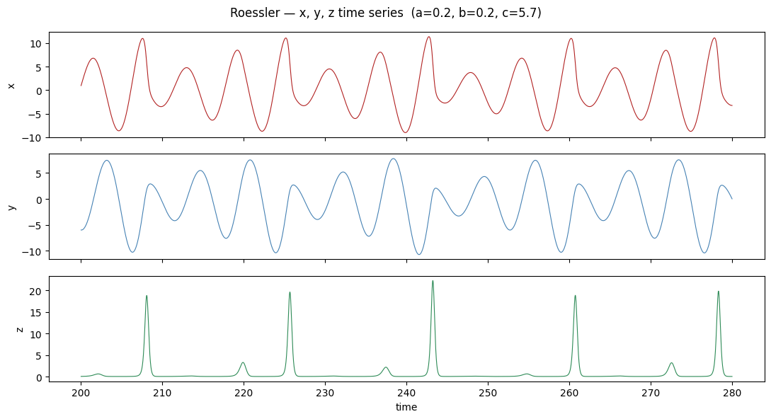

Figure. \(x\) and \(y\) oscillate in approximate anti-phase at the slow frequency. \(z\) is near zero for most of the cycle, then spikes sharply upward when the \((x, y)\) trajectory reaches the outer edge of the spiral. Each \(z\)-spike slightly perturbs the next orbit — this sensitive amplification of small differences is the source of chaos.

Effect of c — periodic to chaotic transition

c controls the dominant dynamics. Below c ≈ 4.2 the attractor is periodic; above that period-doubling cascades to chaos by c ≈ 5.7.

c_cases = [
    (3.5, 'Period-1  (c=3.5)',  'steelblue'),
    (4.1, 'Period-2  (c=4.1)',  'goldenrod'),
    (5.7, 'Chaos     (c=5.7)',  'firebrick'),
]

fig, axes = plt.subplots(1, 3, figsize=(14, 4))

for ax, (c_val, label, color) in zip(axes, c_cases):
    m = Roessler(c=c_val)
    out = m.integrate(t_span=(0, 400), y0=[0.1, 0.0, 0.0], method='RK45')
    xv = out.state_variables['x']
    zv = out.state_variables['z']
    tv = np.asarray(out.time)
    mk = tv > 200
    ax.plot(xv[mk], zv[mk], lw=0.3, color=color, alpha=0.8)
    ax.set_xlabel('x'); ax.set_ylabel('z')
    ax.set_title(label)

fig.suptitle('Roessler — x–z attractor for varying c  (a=0.2, b=0.2)')
plt.tight_layout(); plt.show()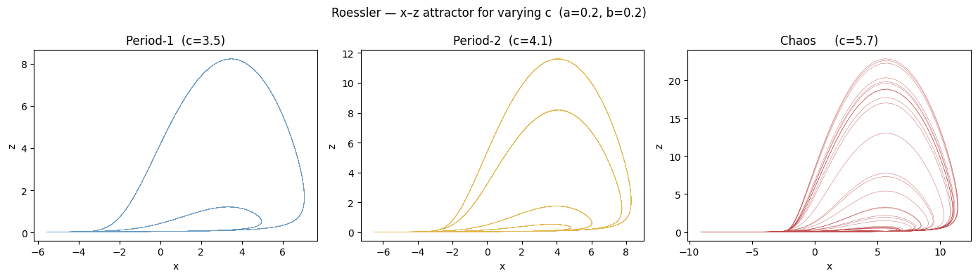

Figure. x–z attractor for three values of \(c\). Period-1 (\(c=3.5\)): a single closed orbit — the trajectory retraces the same path every cycle. Period-2 (\(c=4.1\)): the orbit has split into two nested loops; every other revolution is slightly larger, doubling the period. Chaos (\(c=5.7\)): no two loops are the same; the band has thickened into a continuous sheet characteristic of a strange attractor.

Solver notes

RK45 is appropriate. The Rössler system is not stiff at canonical parameters.

t_span must start at 0 or later. Like Lorenz63, this model accumulates state in dydt using a if t > 0 guard. Negative start times leave a gap in the output.

Discard a transient (first ~100 time units) before taking attractor statistics — the trajectory may start far from the attractor depending on the initial condition.