import numpy as np
import matplotlib.pyplot as plt
import climatecritters as cc
from climatecritters.model_critters.g24 import Model3, calc_f, vc_funcG24 — Ganopolski (2024) Glacial Cycle Model
Abstract
Model3 implements the nonlinear glacial cycle model of Ganopolski (2024), driven by precession-based orbital forcing with eccentricity-modulated amplitude. Discrete regime switching between glaciation and deglaciation modes reproduces ~100 kyr cycles, and a time-varying critical ice-volume threshold vc(t) replicates the Mid-Pleistocene Transition from ~40 kyr to ~100 kyr periodicity.
Keywords
Model3, glacial cycles, orbital forcing, precession, eccentricity, regime switching, ice volume, Mid-Pleistocene Transition, termination, Ganopolski 2024
Overview
Model3 implements the nonlinear threshold model of glacial cycles from Ganopolski (2024). It tracks normalised ice volume v and a discrete glacial regime k (1 = glaciation, 2 = deglaciation). Orbital forcing f(t) drives transitions between regimes.
Equations
Glaciation phase (k = 1): ice volume relaxes toward a forcing-dependent equilibrium \[\frac{dv}{dt} = \frac{v_e(f) - v}{\tau_1}\]
Deglaciation phase (k = 2): rapid, constant-rate collapse \[\frac{dv}{dt} = -\frac{v_c}{\tau_2}\]
Regime switches
| Transition | Condition |
|---|---|
| k=1 → k=2 (termination onset) | v > v_c and df/dt > 0 and f > 0 |
| k=2 → k=1 (glaciation onset) | f < f_1 |
Parameters
| Name | Description | Default |
|---|---|---|
f1 |
Insolation threshold for glaciation onset (W m⁻²) | −16 |
f2 |
Upper insolation threshold (W m⁻²) | 16 |
t1 |
Glaciation relaxation timescale (kyr) | 30 |
t2 |
Deglaciation timescale (kyr) | 10 |
vc |
Critical ice volume for termination trigger | 1.4 |
All parameters accept a float, callable (t) / (t, state), or cc.Forcing.
State variables: v (normalised ice volume), k (regime index, non-integrated).
Diagnostic: insolation — the applied orbital forcing value f(t) at each output step.
Basic run
# Instantiate with default parameters (f1=-16, f2=16, t1=30, t2=10, vc=1.4)
model = Model3()

# Orbital forcing must be registered — it is time-varying, not a static scalar
model.register_forcing('insolation', cc.Forcing(calc_f))

# max_step=0.5 kyr is critical: regime switches (k=1↔2) are discrete events
# inside dydt. An adaptive solver with large steps can stride over a switch
# condition, missing terminations entirely.
output = model.integrate(t_span=(-2000, 0), y0=[0.0, 1], method='RK45',
                         kwargs={'max_step': 0.5})
/Users/jlanders/PycharmProjects/ClimateCritters/climatecritters/model_critters/g24.py:213: RuntimeWarning: invalid value encountered in sqrt
return 1 + np.sqrt((f2 - f) / (f2 - f1))
/Users/jlanders/PycharmProjects/ClimateCritters/climatecritters/model_critters/g24.py:232: RuntimeWarning: invalid value encountered in sqrt
return 1 - np.sqrt((f2 - f) / (f2 - f1))v = output.state_variables['v']
k = output.state_variables['k']
insolation = output.diagnostic_variables['insolation']
time = output.time
# Count terminations (1→2 transitions in k)
n_term = int(np.sum(np.diff(k) > 0))
print(f"Terminations in 2000 kyr: {n_term} (mean cycle ~{2000 / n_term:.0f} kyr)")
print(f"Max ice volume: {v.max():.2f}")
fig, axes = plt.subplots(3, 1, figsize=(11, 7), sharex=True)
# Insolation forcing — drives regime switches
axes[0].plot(time, insolation, color='goldenrod', lw=0.8)
axes[0].axhline(0, color='k', lw=0.5, ls=':')
axes[0].set_ylabel('f (W m\u207b\u00b2)'); axes[0].set_title('Orbital forcing f(t)')
# Ice volume — sawtooth: slow glaciation, rapid termination
axes[1].plot(time, v, color='steelblue', lw=1)
axes[1].axhline(model.vc, color='gray', ls='--', lw=0.8, label=f'vc = {model.vc}')
axes[1].set_ylabel('v (normalised)'); axes[1].set_title('Ice volume')
axes[1].legend(fontsize=9)
# Regime: 1 = glaciation (building), 2 = deglaciation (termination)
axes[2].step(time, k, color='purple', lw=1, where='post')
axes[2].set_yticks([1, 2])
axes[2].set_yticklabels(['glaciation\n(k=1)', 'deglaciation\n(k=2)'])
axes[2].set_ylabel('k'); axes[2].set_xlabel('time (kyr)')
axes[2].set_title('Regime')
fig.suptitle(f'G24 default run — 2000 kyr, {n_term} terminations')
for ax in axes:
ax.invert_xaxis() # geological convention: older on right
plt.tight_layout(); plt.show()Terminations in 2000 kyr: 14 (mean cycle ~143 kyr)
Max ice volume: 1.74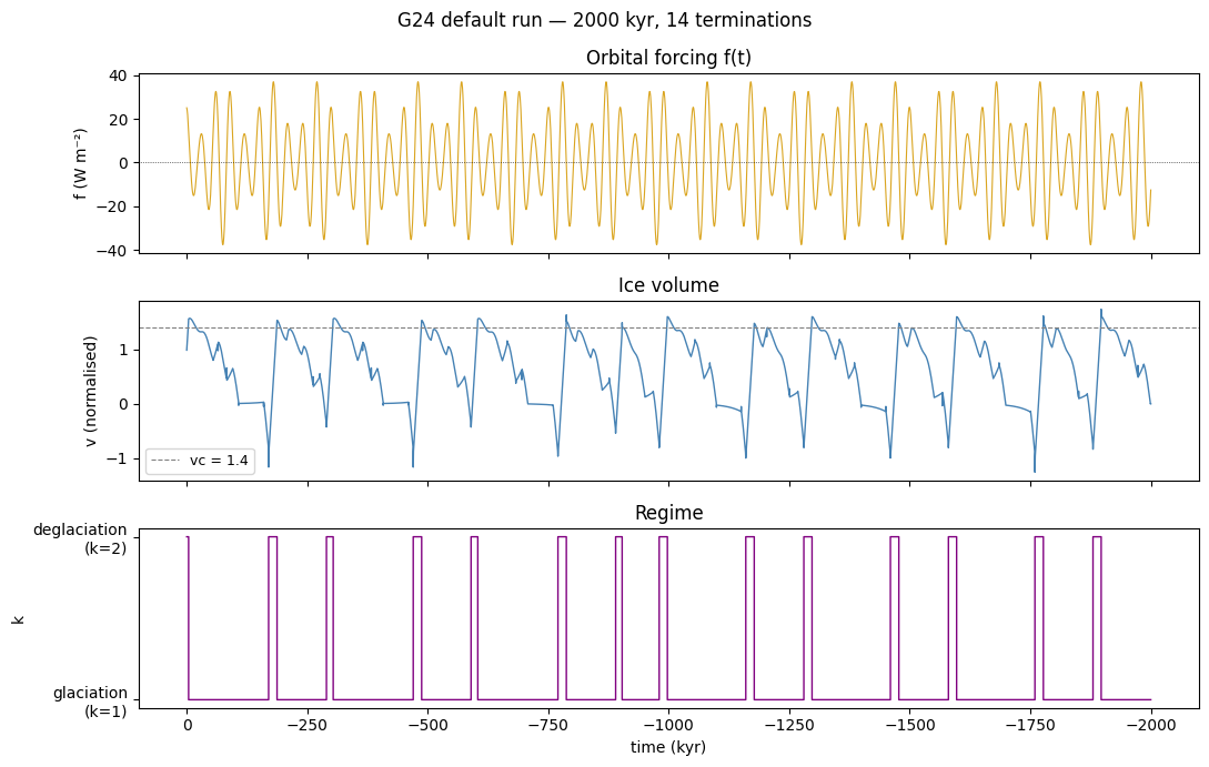
Figure. Top: orbital forcing \(f(t)\) — the signal that drives regime switches. Middle: normalised ice volume \(v\); rises during glaciation, drops sharply at each termination. Bottom: regime state \(k\) (1 = glaciation, 2 = deglaciation). Terminations align with insolation maxima that exceed the deglaciation threshold \(f_2\); the model reproduces ~100 kyr cycles over the last 800 kyr.
Orbital forcing
calc_f provides the Ganopolski (2024) orbital forcing — a precession signal with eccentricity-modulated amplitude:
\[f(t) = A \bigl(1 + \varepsilon\,\sin(2\pi t / T_1)\bigr)\cos(2\pi t / T_2)\]
The \(T_2 = 30\) kyr precession carrier is amplitude-modulated at \(T_1 = 100\) kyr (eccentricity). The result has pronounced 100 kyr amplitude beats — maximal precession peaks during eccentricity maxima.
Register the forcing as a Forcing object so it is evaluated at every solver step:
model.register_forcing('insolation', cc.Forcing(calc_f))# Plot the forcing signal over the last 500 kyr to resolve both precession and eccentricity
t_range = np.linspace(-500, 0, 5000)
f_vals = calc_f(t_range)
fig, ax = plt.subplots(figsize=(11, 3))
ax.plot(t_range, f_vals, color='goldenrod', lw=0.9)
ax.axhline(0, color='k', lw=0.5, ls=':')
ax.set_xlabel('time (kyr)'); ax.set_ylabel('f (W m\u207b\u00b2)')
ax.set_title('calc_f — precession with eccentricity modulation (default parameters)')
ax.invert_xaxis()
plt.tight_layout(); plt.show()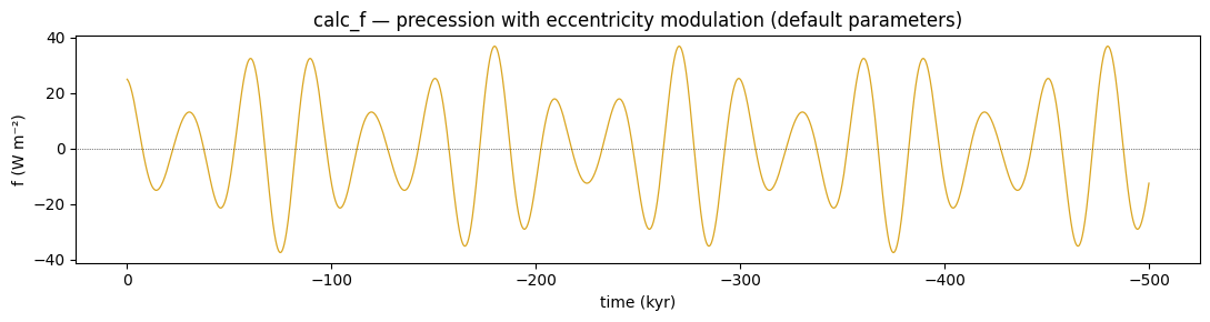
Figure. The calc_f forcing over the last 500 kyr. The signal is dominated by the ~23 kyr precession cycle, with amplitude modulated at ~100 kyr by eccentricity — the beat between consecutive precession cycles is clearly visible near 400 kyr BP.
Forcing parameters
| Parameter | Description | Default |
|---|---|---|
A |
Amplitude (W m⁻²) | 25 |
eps |
Eccentricity modulation depth | 0.5 |
T1 |
Eccentricity period (kyr) | 100 |
T2 |
Precession period (kyr) | 30 |
eps=0 removes the eccentricity envelope, leaving constant-amplitude precession. Comparing the two forcing signals makes the 100 kyr amplitude modulation explicit:
f_eps05 = calc_f(t_range, eps=0.5)   # default: eccentricity modulation on
f_eps0  = calc_f(t_range, eps=0)     # pure precession, constant amplitude

fig, axes = plt.subplots(2, 1, figsize=(11, 5), sharex=True)
axes[0].plot(t_range, f_eps05, color='goldenrod', lw=0.9)
axes[0].set_ylabel('f (W m\u207b\u00b2)')
axes[0].set_title('eps=0.5 (default) — 100 kyr amplitude beats visible')

axes[1].plot(t_range, f_eps0, color='sienna', lw=0.9)
axes[1].set_ylabel('f (W m\u207b\u00b2)')
axes[1].set_title('eps=0 — constant-amplitude precession only')

for ax in axes:
    ax.axhline(0, color='k', lw=0.5, ls=':')
    ax.invert_xaxis()
axes[1].set_xlabel('time (kyr)')
plt.tight_layout(); plt.show()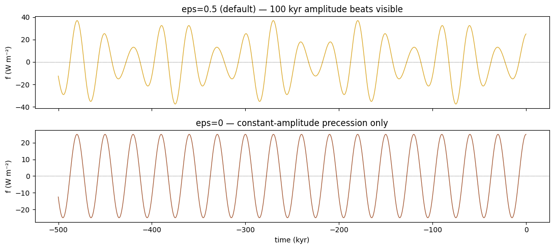
Figure. Top (eps=0.5): eccentricity modulation is on — amplitude waxes and wanes on the 100 kyr eccentricity cycle, producing large and small precession maxima alternately. Bottom (eps=0): pure precession at fixed amplitude. Eccentricity modulation is what intermittently ‘unlocks’ large terminations in the model.
Ice volume threshold: vc
vc is the minimum ice volume required to trigger a termination (k=1 → k=2). It controls both the dominant cycle period and the sawtooth asymmetry:
- Low
vc(≈ 0.65): deglaciation triggers after modest ice build-up → frequent terminations → shorter cycles - High
vc(≈ 1.4): substantial ice build-up required → the system skips forcing beats until enough ice accumulates → longer cycles
The default vc=1.4 reproduces the late Pleistocene 100-kyr world. Note that the calc_f forcing is purely precession-based (no obliquity), so minimum cycle lengths are set by the glaciation timescale t1, not the 41-kyr obliquity period.
# Compare three vc values
vc_values = [0.65, 1.0, 1.4]
vc_colors = ['steelblue', 'seagreen', 'firebrick']
vc_runs   = []

for vc_val in vc_values:
    m = Model3(vc=vc_val)
    m.register_forcing('insolation', cc.Forcing(calc_f))
    out = m.integrate(t_span=(-2000, 0), y0=[0.0, 1], method='RK45',
                      kwargs={'max_step': 0.5})
    vc_runs.append((vc_val, out))

for vc_val, out in vc_runs:
    k_out  = out.state_variables['k']
    n_t    = int(np.sum(np.diff(k_out) > 0))
    print(f"vc={vc_val:.2f}: {n_t} terminations  "
          f"(mean cycle ~{2000 / n_t:.0f} kyr)")
/Users/jlanders/PycharmProjects/ClimateCritters/climatecritters/model_critters/g24.py:213: RuntimeWarning: invalid value encountered in sqrt
return 1 + np.sqrt((f2 - f) / (f2 - f1))
/Users/jlanders/PycharmProjects/ClimateCritters/climatecritters/model_critters/g24.py:232: RuntimeWarning: invalid value encountered in sqrt
return 1 - np.sqrt((f2 - f) / (f2 - f1))vc=0.65: 28 terminations (mean cycle ~71 kyr)
vc=1.00: 18 terminations (mean cycle ~111 kyr)
vc=1.40: 14 terminations (mean cycle ~143 kyr)fig, axes = plt.subplots(len(vc_values), 1, figsize=(11, 7), sharex=True)
for ax, (vc_val, out), color in zip(axes, vc_runs, vc_colors):
v_out = out.state_variables['v']
ax.plot(out.time, v_out, color=color, lw=0.9)
# Dashed line shows the vc threshold each run must cross to deglaciate
ax.axhline(vc_val, color=color, ls='--', lw=0.8, alpha=0.6)
ax.set_ylabel('v')
ax.set_title(f'vc = {vc_val}', loc='left')
ax.invert_xaxis()
axes[-1].set_xlabel('time (kyr)')
fig.suptitle('vc controls dominant periodicity — same forcing, same initial condition')
plt.tight_layout(); plt.show()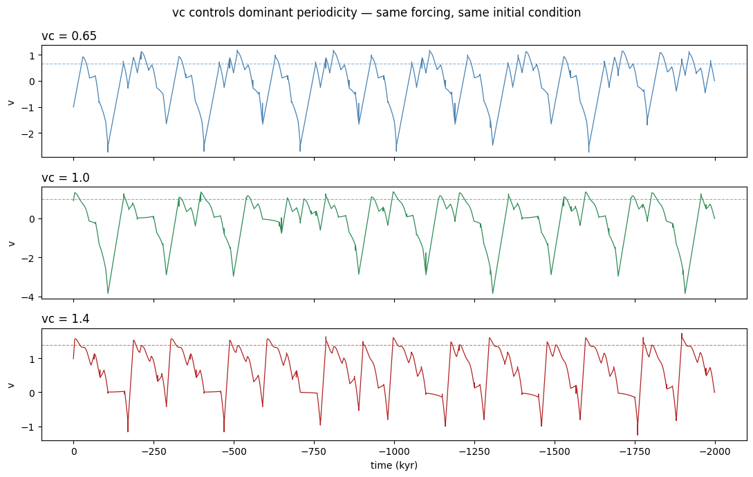
Figure. Ice volume \(v(t)\) for three values of \(v_c\). Low \(v_c=0.65\): terminations trigger readily — short, ~40 kyr obliquity-paced cycles. Middle \(v_c=1.0\): some precession cycles are ‘skipped’, yielding irregular 80–100 kyr cycles. High \(v_c=1.4\) (default): only the largest insolation maxima can drive a termination, producing canonical 100 kyr glacial cycles with saw-tooth asymmetry.
Mid-Pleistocene Transition
The Mid-Pleistocene Transition (MPT, ~1.2–0.8 Ma) saw glacial cycles lengthen from ~40 kyr to ~100 kyr with no corresponding change in orbital forcing. In this model the MPT is reproduced by a gradual increase in vc, captured by vc_func — a sigmoid ramp between a pre-MPT and post-MPT value:
\[v_c(t) = \frac{v_{c1} + v_{c2}}{2} + \frac{v_{c2} - v_{c1}}{2}\,\tanh\!\left(\frac{t - t_{\mathrm{MPT}}}{\tau_1}\right)\]
Default: vc1=0.65 (pre-MPT), vc2=1.38 (post-MPT), t_MPT=−1050 kyr, τ₁=250 kyr.
vc_func has keyword arguments beyond t, so it must be wrapped in a lambda before passing as a parameter callable — the dispatcher only accepts signatures (t), (t, state), or (t, state, model):
Model3(vc=lambda t: vc_func(t))# Plot vc_func over the full integration span
t_long = np.linspace(-2500, 0, 5000)
vc_vals = vc_func(t_long)
fig, ax = plt.subplots(figsize=(11, 2.5))
ax.plot(t_long, vc_vals, color='darkslateblue', lw=1.5)
ax.axvline(-1050, color='gray', ls='--', lw=0.8, label='t_MPT = \u22121050 kyr')
ax.set_xlabel('time (kyr)'); ax.set_ylabel('vc')
ax.set_title('vc_func — sigmoid ramp through the Mid-Pleistocene Transition')
ax.invert_xaxis(); ax.legend()
plt.tight_layout(); plt.show()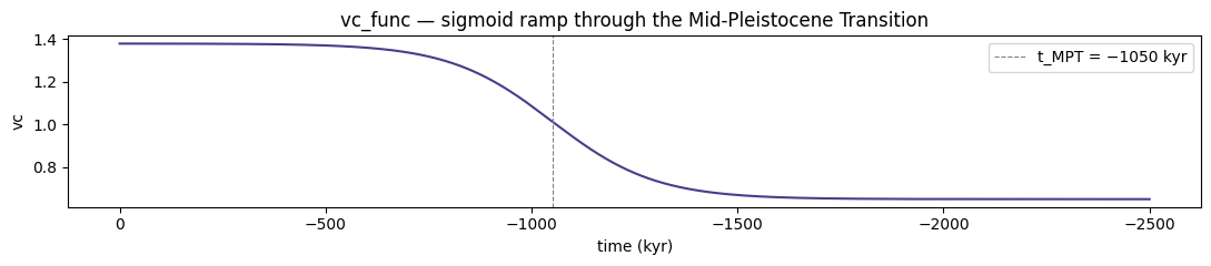
Figure. The sigmoid \(v_c(t)\) ramp used to model the MPT. Before ~1.2 Ma \(v_c\) is low (obliquity world), after ~0.8 Ma it is high (eccentricity world); the transition is smoothed over ~400 kyr.
# vc_func has keyword args (vc1, vc2, ...) beyond t, so wrap it in a lambda.
# The parameter dispatcher only accepts (t), (t, state), or (t, state, model).
model_mpt = Model3(vc=lambda t: vc_func(t))
model_mpt.register_forcing('insolation', cc.Forcing(calc_f))
out_mpt = model_mpt.integrate(t_span=(-2500, 0), y0=[0.0, 1], method='RK45',
                               kwargs={'max_step': 0.5})

v_mpt    = out_mpt.state_variables['v']
k_mpt    = out_mpt.state_variables['k']
time_mpt = out_mpt.time

# Count terminations before and after the MPT centre
pre  = time_mpt < -1050
post = time_mpt > -1050
n_pre  = int(np.sum(np.diff(k_mpt[pre])  > 0))
n_post = int(np.sum(np.diff(k_mpt[post]) > 0))
print(f"Pre-MPT  terminations: {n_pre}   (~{1450 / max(n_pre, 1):.0f} kyr mean cycle)")
print(f"Post-MPT terminations: {n_post}  (~{1050 / max(n_post, 1):.0f} kyr mean cycle)")
Pre-MPT terminations: 23 (~63 kyr mean cycle)
Post-MPT terminations: 8 (~131 kyr mean cycle)fig, axes = plt.subplots(2, 1, figsize=(11, 6), sharex=True)
# vc(t) on top — the evolving threshold
axes[0].plot(t_long, vc_vals, color='darkslateblue', lw=1.2)
axes[0].axvline(-1050, color='gray', ls='--', lw=0.8)
axes[0].set_ylabel('vc')
axes[0].set_title('Critical ice volume vc(t)')
# Ice volume — shorter cycles before MPT, longer after
axes[1].plot(time_mpt, v_mpt, color='steelblue', lw=0.9)
axes[1].axvline(-1050, color='gray', ls='--', lw=0.8, label='t_MPT = \u22121050 kyr')
axes[1].set_ylabel('v (normalised)'); axes[1].set_xlabel('time (kyr)')
axes[1].set_title('Ice volume — shorter cycles \u2192 longer cycles after MPT')
axes[1].legend()
for ax in axes:
ax.invert_xaxis()
fig.suptitle('Mid-Pleistocene Transition with vc_func')
plt.tight_layout(); plt.show()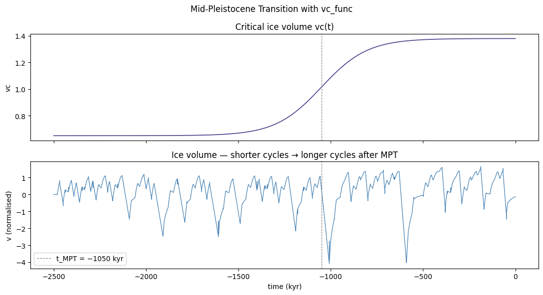
Figure. Top: the evolving \(v_c\) threshold. Bottom: simulated ice volume over 2500 kyr. Before ~1 Ma the model produces rapid ~40 kyr cycles (low threshold, obliquity-forced). After the MPT, \(v_c\) rises and the system skips forcing beats, locking into the longer ~100 kyr rhythm seen in the Pleistocene record.
Glaciation and deglaciation thresholds: f1 and f2
f1 controls when deglaciation ends and glaciation resumes: k=2 → k=1 when f < f1. More negative f1 means insolation must drop further before glaciation can restart, extending the deglaciation phase and altering cycle asymmetry.
f2 defines the upper end of the bi-stable regime. For f1 < f < f2 the equilibrium ice volume ve depends on whether the current v is above or below the unstable equilibrium vu — both the interglacial (ve = 0) and glacial (ve = vg) attractors exist simultaneously in this window.
# Compare three f1 values — all else default (vc=1.4)
f1_values = [-10, -16, -25]
f1_colors = ['steelblue', 'seagreen', 'firebrick']
f1_runs   = []

for f1_val in f1_values:
    m = Model3(f1=f1_val)
    m.register_forcing('insolation', cc.Forcing(calc_f))
    out = m.integrate(t_span=(-1000, 0), y0=[0.0, 1], method='RK45',
                      kwargs={'max_step': 0.5})
    f1_runs.append((f1_val, out))
    k_out = out.state_variables['k']
    n_t   = int(np.sum(np.diff(k_out) > 0))
    print(f"f1={f1_val:>4}: {n_t} terminations in 1000 kyr  "
          f"(mean cycle ~{1000 / max(n_t, 1):.0f} kyr)")
f1= -10: 10 terminations in 1000 kyr (mean cycle ~100 kyr)
f1= -16: 7 terminations in 1000 kyr (mean cycle ~143 kyr)
f1= -25: 5 terminations in 1000 kyr (mean cycle ~200 kyr)fig, axes = plt.subplots(len(f1_values), 1, figsize=(11, 7), sharex=True)
for ax, (f1_val, out), color in zip(axes, f1_runs, f1_colors):
v_out = out.state_variables['v']
ax.plot(out.time, v_out, color=color, lw=1)
ax.axhline(1.4, color='gray', ls=':', lw=0.8) # vc reference
ax.set_ylabel('v')
ax.set_title(f'f1 = {f1_val}', loc='left')
ax.invert_xaxis()
axes[-1].set_xlabel('time (kyr)')
fig.suptitle('Effect of f1 threshold (last 1000 kyr, vc=1.4)')
plt.tight_layout(); plt.show()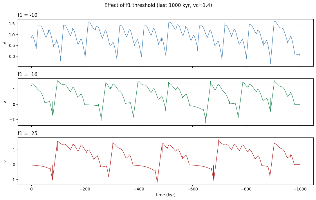
Figure. Ice volume for three deglaciation restart thresholds \(f_1\). High \(f_1=-10\) (less negative): glaciation resumes at a relatively high insolation value — cycles are shorter and more frequent. Low \(f_1=-25\): the system stays in the interglacial state longer, producing extended warm periods and occasional cycle skipping. \(f_1=-16\) (default) gives a good balance between termination frequency and cycle length.
Solver notes
max_step=0.5 kyr is required. Regime switches (k=1↔︎2) are discrete events evaluated inside dydt. An adaptive solver with unrestricted step size can stride over a switch condition, silently missing terminations. Always pass kwargs={'max_step': 0.5}.
Time is in kyr; negative = past (ka BP). t_span=(-2000, 0) runs from 2000 ka to the present.
Initial condition y0=[v0, k0]: v0=0.0 starts ice-free; k0=1 starts in the glaciation phase. Starting with k0=2 (deglaciation) and v0=0 produces an immediate spurious termination.
k is non-integrated. The ODE solver only integrates v. The regime index k is updated in-place inside dydt and stored alongside v in the output’s state variable array.
Callable parameters must have signature (t), (t, state), or (t, state, model). The dispatcher counts all positional arguments, including those with defaults. Functions with keyword-only defaults like vc_func(t, vc1=..., vc2=...) must be wrapped:
Model3(vc=lambda t: vc_func(t))