Stommel — Two-Box Thermohaline Circulation Model

Abstract

Stommel models Atlantic overturning circulation as two boxes — equatorial and polar — exchanging heat and salinity driven by their density contrast. This notebook demonstrates freshwater perturbation via both parameter replacement and state-additive forcing, the bifurcation between thermally-driven and salinity-dominated overturning modes, and time-evolving parameter sweeps.

Keywords

Stommel, thermohaline circulation, AMOC, overturning, freshwater forcing, bistability, salinity-driven mode, density contrast, bifurcation, register_forcing

Overview

The Stommel (1961) model tracks two state variables — the pole-to-equator temperature contrast T and salinity contrast S — and uses them to compute an overturning circulation strength q. Both variables are dimensionless in the default parameter set.

The diagnostic q is the key output: positive values indicate thermally-driven (on) circulation; negative values indicate haline-driven (reversed) circulation.

Equations

\[ q = k(\alpha T - \beta S) \]

\[ \frac{dT}{dt} = -\lambda_T (T - T^*) - |q|\, T \]

\[ \frac{dS}{dt} = E - \lambda_S (S - S^*) - |q|\, S \]

The restoring terms pull T and S toward their equatorial references. The advective terms |q|T and |q|S represent overturning transport. E is a net freshwater flux (evaporation minus precipitation).

Parameters

Name	Description	Default
alpha	Thermal expansion coefficient	1.0
beta	Haline contraction coefficient	1.0
k	Hydraulic constant (sensitivity of q to density contrast)	1.0
E	Net evaporation-minus-precipitation freshwater flux	0.0
lambda_T	Thermal restoring rate	1.0
lambda_S	Saline restoring rate	1.0
T_star	Equilibrium temperature contrast	1.0
S_star	Equilibrium salinity contrast	0.0

All parameters accept a float, a callable (t) / (t, state), or a cc.Forcing object. External forcings are attached after construction via register_forcing — see the Forcing section below.

Basic run

import numpy as np
import matplotlib.pyplot as plt
import climatecritters as cc
from climatecritters.model_critters.stommel import Stommel

model = Stommel(E=0.3, T_star=1.0, S_star=0.0)
output = model.integrate(t_span=(0, 50), y0=[1.0, 0.0], method='RK45')

State variables and the overturning diagnostic are accessed directly from the output object:

T = output.state_variables['T']
S = output.state_variables['S']
q = output.diagnostic_variables['q']
time = output.time

fig, axes = plt.subplots(3, 1, figsize=(8, 7), sharex=True)
axes[0].plot(time, T, color='firebrick');  axes[0].set_ylabel('T')
axes[1].plot(time, S, color='steelblue'); axes[1].set_ylabel('S')
axes[2].plot(time, q, color='purple')
axes[2].axhline(0, color='k', lw=0.8, ls='--')
axes[2].set_ylabel('q (overturning)'); axes[2].set_xlabel('time')
fig.suptitle('Stommel — E=0.3'); plt.tight_layout(); plt.show()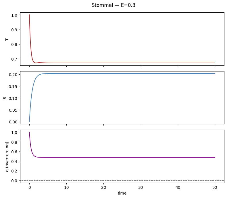

Figure. Default run (\(E=0.3\), \(T^*=1\)). Temperature contrast \(T\) equilibrates quickly (fast restoring). Salinity contrast \(S\) evolves more slowly under the specified freshwater exchange. Overturning \(q\) starts positive (temperature-driven, TH mode) and settles to a steady value — the system remains in the thermally-direct circulation state for these parameters.

Forcing

Forcings are attached after construction using register_forcing. There are two meaningfully different places to attach a freshwater forcing in this model, with different physical interpretations.

First, build the forcing object. cc.Forcing accepts a callable, an array with a time axis, or a sequence of composable Hold, Ramp, and Harmonic elements:

fw_forcing = cc.Forcing.from_sequence([
    cc.forcing.Hold(duration=10, value=0.0),
    cc.forcing.Ramp(duration=5,  y0=0.0, yf=0.5),
    cc.forcing.Hold(duration=15, value=0.5),
    cc.forcing.Ramp(duration=5,  y0=0.5, yf=0.0),
    cc.forcing.Hold(duration=15, value=0.0),
])

Always plot the forcing first so the signal is explicit before running any model:

t_plot = np.linspace(0, 50, 500)
fig, ax = plt.subplots(figsize=(8, 2.5))
ax.plot(t_plot, [fw_forcing.get_forcing(t) for t in t_plot], color='teal')
ax.set_xlabel('time'); ax.set_ylabel('freshwater flux'); ax.set_title('Freshwater pulse forcing')
plt.tight_layout(); plt.show()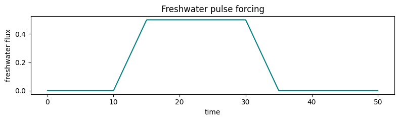

Approach 1: parameter replacement on E

register_forcing('E', forcing_obj) replaces the E parameter entirely with the forcing value at each timestep. This is the natural physical interpretation: the forcing is the freshwater flux. Any value of E set at construction is overridden during integration.

m_E = Stommel(E=0.0, T_star=1.0, S_star=0.0)
m_E.register_forcing('E', fw_forcing)    # attachment_style='replacement', timing='pre' by default
out_E = m_E.integrate(t_span=(0, 50), y0=[1.0, 0.0], method='RK45')

Approach 2: additive forcing on state variable S

register_forcing('S', forcing_obj, 'additive', timing='pre') adds the forcing value to dS/dt inside the right-hand side at each function evaluation. This is a perturbation on top of whatever E is already doing.

m_S = Stommel(E=0.0, T_star=1.0, S_star=0.0)
m_S.register_forcing('S', fw_forcing, 'additive', timing='pre')
out_S = m_S.integrate(t_span=(0, 50), y0=[1.0, 0.0], method='RK45')

Comparing the two approaches

When E=0 at construction, both approaches are mathematically equivalent: replacing E with F(t) gives dS/dt = F(t) - ..., and adding F(t) to dS/dt with E=0 gives the same expression.

t_plot = np.linspace(0, 50, 500)

fig, axes = plt.subplots(3, 1, figsize=(9, 8), sharex=True)

axes[0].plot(t_plot, [fw_forcing.get_forcing(t) for t in t_plot], color='teal')
axes[0].set_ylabel('forcing value'); axes[0].set_title('Applied freshwater signal')

axes[1].plot(out_E.time, out_E.diagnostic_variables['q'],
             color='purple', lw=2, label='E replacement (E=0 base)')
axes[1].plot(out_S.time, out_S.diagnostic_variables['q'],
             color='orange', lw=1.5, ls='--', label='S additive pre (E=0 base)')
axes[1].axhline(0, color='k', lw=0.8, ls=':')
axes[1].set_ylabel('q (overturning)'); axes[1].legend(fontsize=9)

axes[2].plot(out_E.time, out_E.state_variables['S'],
             color='steelblue', lw=2, label='E replacement')
axes[2].plot(out_S.time, out_S.state_variables['S'],
             color='coral', lw=1.5, ls='--', label='S additive pre')
axes[2].set_ylabel('S'); axes[2].set_xlabel('time'); axes[2].legend(fontsize=9)

fig.suptitle('E=0 baseline: both approaches are equivalent', y=1.01)
plt.tight_layout(); plt.show()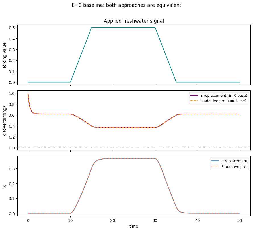

Figure. With \(E=0\) at construction, both forcing approaches are equivalent: the overturning \(q\) traces are indistinguishable (top panel for E-replacement, overlapping dashes for S-additive). The freshwater pulse briefly weakens overturning; the system recovers when the pulse ends. The forcing itself is shown in the top panel for reference.

The distinction matters when there is a non-zero baseline E. Parameter replacement overrides the baseline entirely during the forced period. Additive pre-step superposes the forcing on top of it:

# E=0.3 baseline — replacement overrides it; additive adds on top
m_E_base = Stommel(E=0.3, T_star=1.0, S_star=0.0)
m_E_base.register_forcing('E', fw_forcing)          # E(t) = fw_forcing, ignoring 0.3

m_S_base = Stommel(E=0.3, T_star=1.0, S_star=0.0)
m_S_base.register_forcing('S', fw_forcing, 'additive', timing='pre')  # dS/dt gets +fw_forcing ON TOP of E=0.3

out_E_base = m_E_base.integrate(t_span=(0, 50), y0=[1.0, 0.0], method='RK45')
out_S_base = m_S_base.integrate(t_span=(0, 50), y0=[1.0, 0.0], method='RK45')

fig, ax = plt.subplots(figsize=(8, 4))
ax.plot(output.time,    output.diagnostic_variables['q'],
        color='gray', ls='--', label='unforced (E=0.3)')
ax.plot(out_E_base.time, out_E_base.diagnostic_variables['q'],
        color='purple', label='E replacement (forcing replaces E=0.3)')
ax.plot(out_S_base.time, out_S_base.diagnostic_variables['q'],
        color='orange', label='S additive pre (forcing + E=0.3)')
ax.axhline(0, color='k', lw=0.8, ls=':')
ax.set_ylabel('q (overturning)'); ax.set_xlabel('time'); ax.legend(fontsize=9)
ax.set_title('Non-zero baseline: replacement vs. additive diverge')
plt.tight_layout(); plt.show()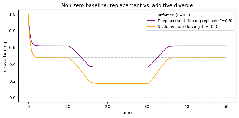

Figure. With \(E=0.3\) at construction, the two approaches diverge. E-replacement: the baseline \(E=0.3\) is completely overridden — during Hold periods E=0, so the effective freshwater input is zero. S-additive: the forcing adds on top of the existing \(E=0.3\) term in \(\dot{S}\), so the total freshwater influence is \(E + f(t)\). Choose the approach that matches the physical interpretation of your forcing.

Summary of the two approaches:

	register_forcing('E', ...)	register_forcing('S', ..., 'additive', timing='pre')
Acts on	parameter E in param_values	state variable S via dS/dt
With non-zero E	replaces the baseline entirely	adds perturbation on top of baseline
Physical meaning	the forcing is the net freshwater flux	an additional flux injected into the salinity budget
With adaptive solver (RK45)	✓ applied at every function evaluation	✓ applied at every function evaluation

Note on timing='post': Registering a state-variable additive forcing with timing='post' would add the forcing value directly to S after each integration step (rather than to dS/dt). This is not physically meaningful here and will generate a warning when used with adaptive solvers, which do not support post-step application.

Time-evolving parameters

Any parameter in param_values can be a callable instead of a scalar. The dispatcher accepts (t), (t, state), or (t, state, model). Here E drifts upward slowly without using a Forcing object:

def E_ramp(t):
    return np.clip(0.012 * t, 0.0, 0.6)

model_ramp = Stommel(E=E_ramp, T_star=1.0, S_star=0.0)
out_ramp = model_ramp.integrate(t_span=(0, 50), y0=[1.0, 0.0], method='RK45')

fig, axes = plt.subplots(2, 1, figsize=(8, 5), sharex=True)
axes[0].plot(out_ramp.time, out_ramp.diagnostic_variables['q'], color='purple')
axes[0].axhline(0, color='k', lw=0.8, ls='--'); axes[0].set_ylabel('q')
t_plot = np.linspace(0, 50, 500)
axes[1].plot(t_plot, [E_ramp(t) for t in t_plot], color='teal')
axes[1].set_ylabel('E(t)'); axes[1].set_xlabel('time')
plt.tight_layout(); plt.show()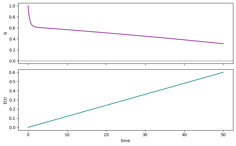

Figure. Top: overturning \(q\) under a linearly increasing \(E\) (freshwater input). \(q\) declines steadily and crosses zero around \(t \approx 35\) — the circulation collapses from thermally-direct (TH mode, \(q>0\)) to salinity-driven (SA mode, \(q<0\)). Bottom: the \(E(t)\) ramp used. This is the canonical Stommel bifurcation: once \(q<0\), the system is in a different stable state.

Converting to pyleoclim

ts_q = output.to_pyleo(var_names=['q'])
ts_q.plot()
plt.show()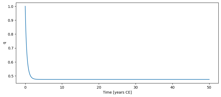

{}

Solver notes

RK45 is appropriate for this model. Near an overturning collapse (where q passes through zero) the system can stiffen — tighten tolerances if trajectories look erratic:

output = model.integrate(
    t_span=(0, 50), y0=[1.0, 0.0], method='RK45',
    kwargs={'rtol': 1e-8, 'atol': 1e-10},
)

The diagnostic q is computed from the full trajectory after integration (uses_post_history = True) and is not available mid-run.