DoublePendulum — Conservative Chaos

Author

Jordan Landers

Published

June 12, 2026

Abstract

DoublePendulum is an energy-conserving (Hamiltonian) system that exhibits deterministic chaos without any dissipation. This notebook demonstrates sensitive dependence on initial conditions, exponential trajectory divergence, and the tradeoff between energy conservation and solver tolerance — contrasting conservative chaos with the dissipative chaos of driven systems.

Keywords

DoublePendulum, Hamiltonian, conservative chaos, energy conservation, sensitive dependence, trajectory divergence, solver tolerance, phase space, Lyapunov

Overview

DoublePendulum implements two point masses on rigid, massless rods swinging from a fixed pivot. The system is Hamiltonian (energy-conserving) with no damping by default, and is chaotic for most non-trivial initial conditions.

Equations

\[\frac{d\theta_1}{dt} = \omega_1 \qquad \frac{d\theta_2}{dt} = \omega_2\]

\[\frac{d\omega_1}{dt} = \frac{-g(2m_1+m_2)\sin\theta_1 - m_2 g\sin(\theta_1-2\theta_2)- 2\sin\Delta\,m_2(\omega_2^2 L_2 + \omega_1^2 L_1\cos\Delta)}{L_1[2m_1+m_2-m_2\cos 2\Delta]} - d_1\omega_1\]

\[\frac{d\omega_2}{dt} = \frac{2\sin\Delta(\omega_1^2 L_1(m_1+m_2) + g(m_1+m_2)\cos\theta_1 + \omega_2^2 L_2 m_2\cos\Delta)}{L_2[2m_1+m_2-m_2\cos 2\Delta]} - d_2\omega_2\]

where \(\Delta = \theta_1 - \theta_2\).

Parameters

Name	Description	Default
`m1`, `m2`	Bob masses (kg)	1.0, 1.0
`L1`, `L2`	Rod lengths (m)	1.0, 1.0
`g`	Gravitational acceleration (m/s²)	9.81
`d1`, `d2`	Linear damping on each bob (s⁻¹)	0.0, 0.0

State variables: theta1, omega1, theta2, omega2. Diagnostics: energy, x1, y1, x2, y2 (Cartesian positions, pivot at origin).

import numpy as np
import matplotlib.pyplot as plt
from climatecritters.model_critters.pendulum import DoublePendulum

Basic run

Starting from a large-amplitude, asymmetric configuration (\(\theta_1 = 120°\), \(\theta_2 = -20°\)) the lower bob traces an irregular path — a hallmark of deterministic chaos.

# θ₁=120°, ω₁=0, θ₂=-20°, ω₂=0 — large amplitude, asymmetric
IC = [2 * np.pi / 3, 0.0, -np.pi / 9, 0.0]

dp = DoublePendulum(m1=1.0, m2=1.0, L1=1.0, L2=1.0, g=9.81)
output = dp.integrate(t_span=(0, 30), y0=IC, method='RK45',
                      kwargs={'rtol': 1e-9, 'atol': 1e-11})

t = np.asarray(output.time)
theta1 = np.degrees(output.state_variables['theta1'])
theta2 = np.degrees(output.state_variables['theta2'])
E0 = output.diagnostic_variables['energy'][0]

print(f'Initial energy E₀ = {E0:.4f} J')
print(f'Steps: {len(t)}')

Initial energy E₀ = 0.5916 J
Steps: 3330

x1 = output.diagnostic_variables['x1']
y1 = output.diagnostic_variables['y1']
x2 = output.diagnostic_variables['x2']
y2 = output.diagnostic_variables['y2']

fig, axes = plt.subplots(1, 3, figsize=(15, 4))

# Angle time series
axes[0].plot(t, theta1, lw=0.8, color='steelblue', label='θ₁  (upper)')
axes[0].plot(t, theta2, lw=0.8, color='firebrick', label='θ₂  (lower)')
axes[0].set_xlabel('time (s)'); axes[0].set_ylabel('angle (°)')
axes[0].set_title('Angular displacement')
axes[0].legend(fontsize=9)

# Bob 2 Cartesian trajectory
sc = axes[1].scatter(x2, y2, c=t, cmap='viridis', s=0.5, lw=0)
axes[1].scatter([x2[0]], [y2[0]], color='lime', s=50, zorder=5, label='start')
axes[1].scatter([x2[-1]], [y2[-1]], color='red',  s=50, zorder=5, label='end')
fig.colorbar(sc, ax=axes[1], label='time (s)')
axes[1].set_xlabel('x₂ (m)'); axes[1].set_ylabel('y₂ (m)')
axes[1].set_title('Bob 2: Cartesian trajectory')
axes[1].set_aspect('equal')
axes[1].legend(fontsize=9)

# θ₁–θ₂ phase portrait
axes[2].plot(theta1, theta2, lw=0.4, color='#333333', alpha=0.8)
axes[2].set_xlabel('θ₁ (°)'); axes[2].set_ylabel('θ₂ (°)')
axes[2].set_title('θ₁–θ₂ configuration space')

fig.suptitle('DoublePendulum — θ₁=120°, θ₂=−20°')
plt.tight_layout(); plt.show()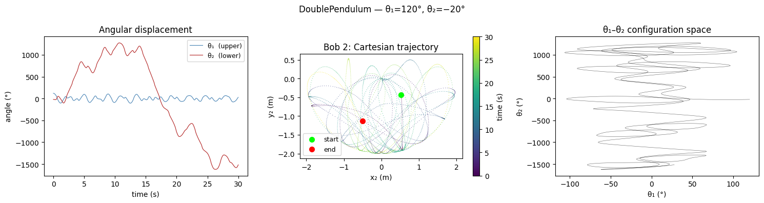

Figure. Starting from \(\theta_1=120°\), \(\theta_2=-20°\). Left: both angles range widely and irregularly — the system never settles. Centre: the lower bob’s Cartesian path densely fills a region of space with no apparent pattern. Right: the \((\theta_1, \theta_2)\) configuration portrait traces a space-filling curve that never closes — the signature of conservative chaos in a Hamiltonian system.

Sensitive dependence on initial conditions

Two trajectories starting \(\varepsilon = 10^{-6}\) rad apart in \(\theta_1\) diverge exponentially and become fully uncorrelated within a few seconds.

eps = 1e-6
kw_tight = {'rtol': 1e-10, 'atol': 1e-12}

dp_a = DoublePendulum()
out_a = dp_a.integrate(t_span=(0, 20), y0=IC, method='RK45', kwargs=kw_tight)

IC_perturbed = [IC[0] + eps, IC[1], IC[2], IC[3]]
dp_b = DoublePendulum()
out_b = dp_b.integrate(t_span=(0, 20), y0=IC_perturbed, method='RK45', kwargs=kw_tight)

t_a = np.asarray(out_a.time)
t_b = np.asarray(out_b.time)

# Interpolate b onto a's time grid for pointwise comparison
th1_b_interp = np.interp(t_a, t_b, out_b.state_variables['theta1'])
th2_b_interp = np.interp(t_a, t_b, out_b.state_variables['theta2'])
om1_b_interp = np.interp(t_a, t_b, out_b.state_variables['omega1'])
om2_b_interp = np.interp(t_a, t_b, out_b.state_variables['omega2'])

sep = np.sqrt(
    (out_a.state_variables['theta1'] - th1_b_interp)**2 +
    (out_a.state_variables['theta2'] - th2_b_interp)**2 +
    (out_a.state_variables['omega1'] - om1_b_interp)**2 +
    (out_a.state_variables['omega2'] - om2_b_interp)**2
)

fig, axes = plt.subplots(1, 2, figsize=(12, 4))

axes[0].plot(t_a, np.degrees(out_a.state_variables['theta1']),
             lw=0.8, color='steelblue', label='Original')
axes[0].plot(t_b, np.degrees(out_b.state_variables['theta1']),
             lw=0.8, color='firebrick', alpha=0.7, label=f'Perturbed (ε={eps:.0e} rad)')
axes[0].set_xlabel('time (s)'); axes[0].set_ylabel('θ₁ (°)')
axes[0].set_title('Upper bob angle — diverge after ~5 s')
axes[0].legend(fontsize=9)

axes[1].semilogy(t_a, sep + 1e-18, lw=1.0, color='#333333')
axes[1].axhline(1.0, color='firebrick', ls='--', lw=0.9, label='O(1) saturation')
axes[1].set_xlabel('time (s)'); axes[1].set_ylabel('phase-space separation')
axes[1].set_title(f'Exponential divergence  (ε={eps:.0e} rad in θ₁)')
axes[1].legend(fontsize=9)

fig.suptitle('DoublePendulum — sensitive dependence on initial conditions')
plt.tight_layout(); plt.show()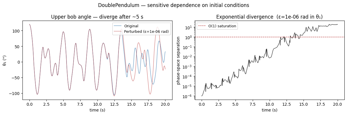

Figure. Left: two trajectories starting \(\varepsilon = 10^{-6}\) rad apart in \(\theta_1\) track each other for ~5 s then diverge completely — indistinguishable early, totally uncorrelated late. Right: phase-space separation on a log scale grows exponentially (positive Lyapunov exponent) then saturates at O(1) once the trajectories are exploring the full attractor independently.

Energy conservation vs solver tolerance

The undamped double pendulum is Hamiltonian — total energy is an exact constant. Relative energy error \(|E(t)-E_0|/|E_0|\) measures integration quality.

tol_cases = [
    ('Default  (rtol=1e-3)', {},                              'firebrick'),
    ('Moderate (rtol=1e-6)', {'rtol': 1e-6, 'atol': 1e-8},   'goldenrod'),
    ('Tight    (rtol=1e-10)',{'rtol': 1e-10,'atol': 1e-12},   'steelblue'),
]

for label, kw, _ in tol_cases:
    m = DoublePendulum()
    out = m.integrate(t_span=(0, 40), y0=IC, method='RK45', kwargs=kw)
    E = out.diagnostic_variables['energy']
    max_err = np.max(np.abs(E - E[0])) / np.abs(E[0])
    print(f'{label:35s}  steps={len(out.time):5d}  max|ΔE/E₀|={max_err:.2e}')

Default  (rtol=1e-3)                 steps=  337  max|ΔE/E₀|=1.58e+01
Moderate (rtol=1e-6)                 steps= 1092  max|ΔE/E₀|=2.26e-03
Tight    (rtol=1e-10)                steps= 7191  max|ΔE/E₀|=1.45e-08

fig, ax = plt.subplots(figsize=(10, 4))

for label, kw, color in tol_cases:
    m = DoublePendulum()
    out = m.integrate(t_span=(0, 40), y0=IC, method='RK45', kwargs=kw)
    E = out.diagnostic_variables['energy']
    ax.semilogy(np.asarray(out.time), np.abs(E - E[0]) / np.abs(E[0]) + 1e-18,
                lw=0.8, color=color, label=label)

ax.set_xlabel('time (s)'); ax.set_ylabel('|ΔE / E₀|')
ax.set_title('Energy conservation error vs RK45 tolerance')
ax.legend(fontsize=9)
plt.tight_layout(); plt.show()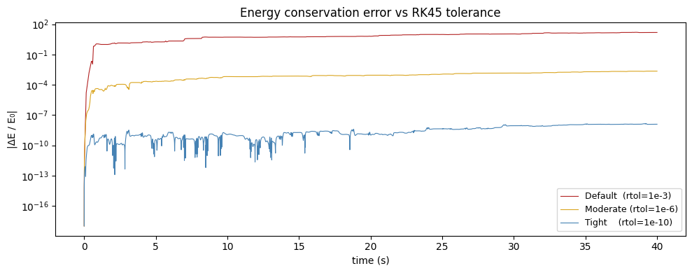

Figure. Relative energy error \(|\Delta E / E_0|\) for three solver tolerances. Default tolerances (rtol=1e-3) accumulate O(10) error — the integrator is taking steps too large to respect the Hamiltonian structure. Moderate tolerances (rtol=1e-6) keep error below 0.2%. Tight tolerances (rtol=1e-10) maintain \(|\Delta E / E_0| < 10^{-8}\) throughout. Use tight tolerances whenever energy conservation or Poincaré sections matter.

Solver notes

RK45 (adaptive) is the recommended solver. Default tolerances are adequate for short qualitative runs; for energy-sensitive diagnostics use tight tolerances:

output = model.integrate(..., kwargs={'rtol': 1e-9, 'atol': 1e-11})

Optional damping: set d1 and/or d2 to positive values to add linear damping on each bob. With damping the system is no longer Hamiltonian and energy decays monotonically.

Cartesian positions (x1, y1, x2, y2) are computed from angles after integration and accessible via output.diagnostic_variables or model.cartesian_positions().

Note: A MultiPendulum class supporting N-rod chains is not yet in the public codebase. For \(N>2\) rods the recommended approach is to subclass DoublePendulum and override dydt using the Lagrangian mass-matrix formulation, solving \(M(\theta)\,\ddot{\theta} = \tau(\theta,\dot{\theta})\) with numpy.linalg.solve at each step.