Solver Selection Guide

Author

Jordan Landers

Published

June 12, 2026

Abstract

Choosing the right numerical integrator matters: adaptive RK45 handles smooth ODEs efficiently but can produce spurious structure at loose tolerances; discrete-event models like G24 require fixed-step solvers to avoid missed threshold crossings; SDE models need stochastic-aware integrators; and two-scale Lorenz96 requires fixed-step rk4 to prevent history corruption. This notebook provides a practical guide with examples and a model-class-to-solver summary table.

Keywords

solver, RK45, rk4, Euler, adaptive, fixed-step, tolerance, discrete-event, SDE, Lorenz96, two-scale, history corruption, timestep

import numpy as np
import matplotlib.pyplot as plt
import climatecritters as cc
from climatecritters.model_critters.ebm import EBM0D, albedo_func
from climatecritters.model_critters.g24 import Model3, calc_f
from climatecritters.model_critters.lorenz import Lorenz96

EBM0D: smooth continuous ODE

EBM0D is a single-variable ODE with no fast processes and a smooth right-hand side — the ideal case for an adaptive solver.

RK45 tolerances

ClimateCritters uses tighter-than-scipy-default tolerances (rtol=1e-8, atol=1e-10) to suppress ghost structure in slow steady-state tails. With scipy defaults the equilibrium temperature can appear to drift by a few mK even after the model has converged.

Run the same integration with both tolerance levels and compare.

model = EBM0D()

# Package-default tight tolerances
out_tight = model.integrate(t_span=(0, 500), y0=[255.0], method='RK45')

# Scipy-default relaxed tolerances (pass empty kwargs to bypass CC defaults)
out_scipy = model.integrate(t_span=(0, 500), y0=[255.0], method='RK45', kwargs={})

T_tight = out_tight.state_variables['T']
T_scipy = out_scipy.state_variables['T']

fig, axes = plt.subplots(1, 2, figsize=(12, 4))

# Full transient
axes[0].plot(out_tight.time, T_tight, color='steelblue', lw=1.5,
             label='RK45 tight (rtol=1e-8)')
axes[0].plot(out_scipy.time, T_scipy, color='firebrick', lw=1, ls='--',
             label='RK45 scipy default')
axes[0].set_xlabel('time (yr)'); axes[0].set_ylabel('T (K)')
axes[0].set_title('Full transient (0–500 yr)'); axes[0].legend()

# Zoom on the equilibrium tail — separate masks per run (adaptive solver step counts differ)
mask_tight = out_tight.time > 400
mask_scipy = out_scipy.time > 400
axes[1].plot(out_tight.time[mask_tight], T_tight[mask_tight], color='steelblue', lw=1.5,
             label='RK45 tight')
axes[1].plot(out_scipy.time[mask_scipy], T_scipy[mask_scipy], color='firebrick', lw=1, ls='--',
             label='RK45 scipy default')
axes[1].set_xlabel('time (yr)'); axes[1].set_ylabel('T (K)')
axes[1].set_title('Equilibrium tail (400–500 yr, zoomed)'); axes[1].legend()

fig.suptitle('EBM0D — RK45 tolerance comparison')
plt.tight_layout(); plt.show()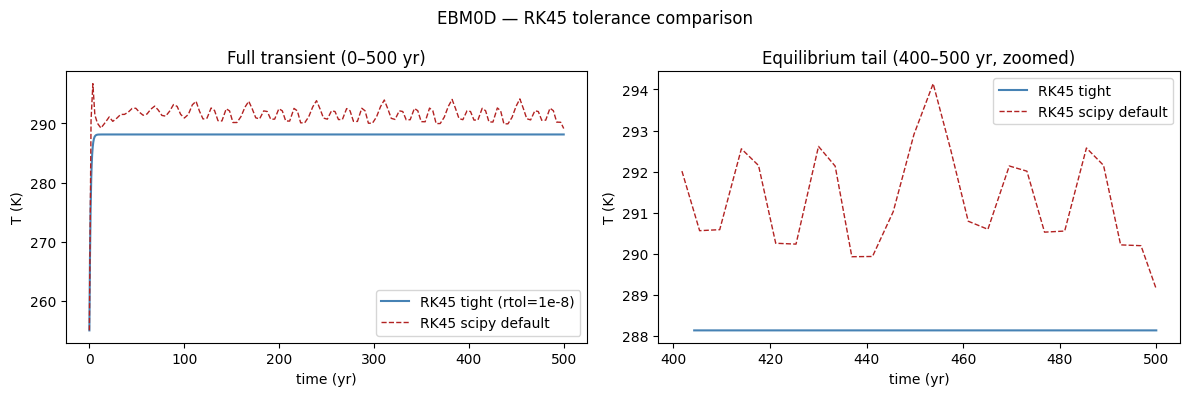

Figure. Left: both runs trace the same transient — tolerance has no visible effect during the fast warm-up. Right (zoomed): with scipy defaults (rtol=1e-3, atol=1e-6) the equilibrium tail shows a few mK of drift that disappears with tight tolerances. For publication-quality figures or bifurcation analyses that compare equilibria, use the package defaults or tighter.

Fixed-step solver: Euler

euler takes a fixed dt and never adapts. It is slower per unit of accuracy than RK45 but has no overhead from step-size control — useful when the right-hand side is cheap or when a specific temporal resolution is required.

model_e = EBM0D()
out_euler = model_e.integrate(t_span=(0, 500), y0=[255.0], method='euler', dt=1.0)
T_euler   = out_euler.state_variables['T']
print(f'Euler T_eq = {T_euler[-1]:.4f} K   RK45 T_eq = {T_tight[-1]:.4f} K')

Euler T_eq = 288.1313 K   RK45 T_eq = 288.1313 K

fig, ax = plt.subplots(figsize=(10, 4))
ax.plot(out_tight.time, T_tight, color='steelblue', lw=2,   label='RK45 (adaptive, tight)')
ax.plot(out_euler.time, T_euler, color='firebrick', lw=1.2, ls='--', label='Euler dt=1.0')
ax.set_xlabel('time (yr)'); ax.set_ylabel('T (K)')
ax.set_title('EBM0D — RK45 vs Euler (dt=1.0 yr)')
ax.legend(); plt.tight_layout(); plt.show()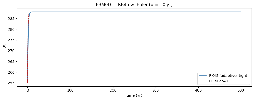

Figure. Both methods converge to the same equilibrium temperature. Euler overshoots the fast early transient slightly and is marginally slower due to the fixed small step, but produces the correct long-run behaviour. RK45 adapts its step size to track the transient efficiently and is the preferred choice for smooth ODEs like EBM0D.

Spurious structure in the transient

With the ice-albedo feedback active (albedo=albedo_func) the EBM0D has two attractors separated by an unstable branch near 260–290 K. Loose solver tolerances don’t change the long-run equilibrium, but they can make the transient look wrong: the solver takes large, inaccurate steps that produce oscillations or apparent excursions toward the opposite branch — structure that does not exist in the true solution. A reader looking only at the transient could mistake a numerical artefact for genuine metastability or bifurcation behaviour.

ICs = [230, 245,251, 258,265, 268,272, 278, 288, 295, 300]   # K
colors = plt.cm.coolwarm(np.linspace(0, 1, len(ICs)))

runs_tight, runs_scipy = [], []
m = EBM0D(albedo=albedo_func)
for T0 in ICs:
    runs_tight.append((T0, m.integrate(t_span=(0, 500), y0=[T0], method='RK45')))
    runs_scipy.append((T0, m.integrate(t_span=(0, 500), y0=[T0], method='RK45', kwargs={})))

fig, axs = plt.subplots(1, 2, figsize=(13, 4), sharey=True)
for ik, (title, run_set) in enumerate([
        ('RK45 tight tolerances', runs_tight),
        ('RK45 scipy defaults',   runs_scipy)]):
    for (T0, out), c in zip(run_set, colors):
        axs[ik].plot(out.time, out.state_variables['T'], color=c, lw=1)
    axs[ik].axhspan(260, 290, alpha=0.07, color='green')
    axs[ik].set_xlabel('time (yr)'); axs[ik].set_title(title)
axs[0].set_ylabel('T (K)')
fig.suptitle('EBM0D with ice-albedo feedback — tolerance vs bistability')
plt.tight_layout(); plt.show()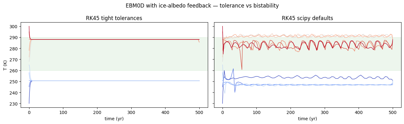

Figure. All trajectories reach the same long-run equilibria regardless of tolerance (warm or cold branch, matching tight tolerances), so the solver configuration has no effect on the answer. The transient is a different matter: with scipy default tolerances (right panel) some trajectories show noisy, irregular paths — including brief apparent excursions toward the opposite branch — that are absent under tight tolerances (left panel). These are solver artefacts, not physics. The shaded band marks the unstable transition zone where the true solution changes direction rapidly; this is exactly where a large step is most likely to mis-evaluate the derivative and introduce spurious structure.

G24: discrete-event ODE

Model3 from Ganopolski (2024) switches between two regime functions at discrete thresholds — the right-hand side is continuous but contains rapid jumps in k (the glaciation/deglaciation state). Adaptive solvers can mis-step across these events and introduce artificial sub-harmonic structure in the ice-volume record.

Fixed-step solvers (Euler, rk4) must be used. The paper uses ~6.5 kyr. This section shows: (1) how Euler and rk4 compare across timesteps, and (2) what happens when you pass RK45 to this model.

g24_forcing = cc.Forcing(calc_f, params={'A': 25, 'eps': 0.5})

f1, f2 = -16.0, 16.0
vc     = 1.4
t1, t2 = 30.0, 10.0
A, eps = 25, 0.5
T_SPAN = (-2000, 0)   # kyr
ZOOM   = (-1000, 0)

delta_ts = [2.0, 4.0, 6.5, 10.0]

runs_euler = {}
for dt in delta_ts:
    m = Model3(vc=vc, f1=f1, f2=f2, t1=t1, t2=t2)
    m.register_forcing('insolation', g24_forcing)
    out = m.integrate(t_span=T_SPAN, y0=[0.0, 1], method='euler', dt=dt)
    runs_euler[dt] = out
    n_term = int(np.sum(np.diff(out.state_variables['k']) > 0))
    print(f'dt={dt:5.1f} kyr  {n_term} terminations  '
          f'(mean {abs(T_SPAN[0])/max(n_term,1):.0f} kyr cycle)')

dt=  2.0 kyr  20 terminations  (mean 100 kyr cycle)
dt=  4.0 kyr  20 terminations  (mean 100 kyr cycle)
dt=  6.5 kyr  19 terminations  (mean 105 kyr cycle)
dt= 10.0 kyr  18 terminations  (mean 111 kyr cycle)

/Users/jlanders/PycharmProjects/ClimateCritters/climatecritters/model_critters/g24.py:213: RuntimeWarning: invalid value encountered in sqrt
  return 1 + np.sqrt((f2 - f) / (f2 - f1))
/Users/jlanders/PycharmProjects/ClimateCritters/climatecritters/model_critters/g24.py:232: RuntimeWarning: invalid value encountered in sqrt
  return 1 - np.sqrt((f2 - f) / (f2 - f1))

colours = ['#2196F3', '#E91E63', '#4CAF50', '#9C27B0']
n = len(delta_ts)

fig = plt.figure(figsize=(13, 11))
# 2 rows per dt: [forcing strip, ice volume] with height ratio 1:2.5
hr = [h for _ in range(n) for h in (1, 2.5)]
gs = fig.add_gridspec(2 * n, 1, hspace=0.1, height_ratios=hr)

for idx, (dt, col) in enumerate(zip(delta_ts, colours)):
    ax_f = fig.add_subplot(gs[2 * idx])
    ax_v = fig.add_subplot(gs[2 * idx + 1], sharex=ax_f)

    out = runs_euler[dt]
    t = out.time
    v = out.state_variables['v']
    k = out.state_variables['k']
    mask = (t >= ZOOM[0]) & (t <= ZOOM[1])
    tm, vm, km = t[mask], v[mask], k[mask]

    # Forcing sampled at this dt's timesteps
    fm = calc_f(tm, A=A, eps=eps)

    # ── Forcing strip ──────────────────────────────────────────────────────
    ax_f.plot(tm, fm, lw=0.8, color=col, alpha=0.7)
    ax_f.scatter(tm, fm, s=2, color=col, alpha=0.5, zorder=3)
    ax_f.axhline(f1, ls='--', color='#888', lw=0.7)   # inception threshold
    ax_f.axhline(f2, ls='--', color='#888', lw=0.7)   # deglaciation threshold
    ax_f.set_ylabel('f', fontsize=7)
    ax_f.tick_params(labelbottom=False, labelsize=7)
    ax_f.set_title(f'dt = {dt} kyr', loc='left', fontsize=9)

    # ── Ice volume ─────────────────────────────────────────────────────────
    in_k2 = False
    for j in range(len(tm)):
        if km[j] == 2 and not in_k2:
            x0 = tm[j]; in_k2 = True
        elif km[j] != 2 and in_k2:
            ax_v.axvspan(x0, tm[j], alpha=0.15, color=col, lw=0)
            in_k2 = False
    if in_k2:
        ax_v.axvspan(x0, tm[-1], alpha=0.15, color=col, lw=0)

    ax_v.plot(tm, vm, lw=0.9, color=col)
    ax_v.axhline(vc, ls='--', color='#888', lw=0.8, alpha=0.6)
    ax_v.set_ylabel('v', fontsize=8)
    ax_v.tick_params(labelsize=8)
    if idx < n - 1:
        ax_v.tick_params(labelbottom=False)

    ax_f.invert_xaxis()

ax_v.set_xlabel('time (kyr)')
fig.suptitle('G24 — Euler timestep sensitivity\nforcing (top strip) and ice volume (bottom) per dt',
             y=1.01)
plt.show()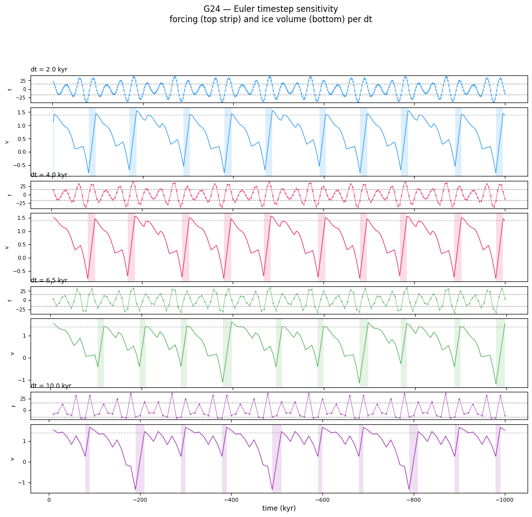

Figure. Each dt group shows: (top) the orbital forcing \(f(t)\) sampled at that timestep — markers indicate the actual evaluation points — with dashed lines at the inception (\(f_1\)) and deglaciation (\(f_2\)) thresholds; (bottom) the resulting ice volume, with deglaciation phases (k = 2) shaded and \(v_c\) dashed.

At dt = 2–4 kyr the forcing is well-resolved: the ~21 kyr precession and ~41 kyr obliquity beats are both captured, and the ice volume shows canonical ~100 kyr saw-tooth cycles. At dt = 6.5 kyr the forcing is marginally resolved; the ~23 kyr precession cycle begins to alias but the 100 kyr rhythm persists. At dt = 10 kyr long gaps between forcing evaluations allow threshold crossings to be stepped over entirely — the model enters or exits a glaciation at the wrong time, producing irregular or shortened cycles.

# Attempt RK45 — adaptive solver on a discontinuous RHS
try:
    m_rk45 = Model3(vc=vc, f1=f1, f2=f2, t1=t1, t2=t2)
    m_rk45.register_forcing('insolation', g24_forcing)
    out_rk45 = m_rk45.integrate(t_span=(-400, 0), y0=[0.0, 1], method='RK45')
    v_rk45 = out_rk45.state_variables['v']
    t_rk45 = out_rk45.time

    fig, axes = plt.subplots(2, 1, figsize=(12, 6), sharex=True)
    ref = runs_euler[2.0]
    mask = (ref.time >= -400) & (ref.time <= 0)
    axes[0].plot(ref.time[mask], ref.state_variables['v'][mask],
                 color='#2196F3', lw=0.9, label='Euler dt=2 kyr (reference)')
    axes[0].axhline(vc, ls='--', color='#888', lw=0.8, alpha=0.6)
    axes[0].set_ylabel('v'); axes[0].legend(fontsize=8); axes[0].invert_xaxis()

    axes[1].plot(t_rk45, v_rk45, color='#E91E63', lw=0.9, label='RK45 (adaptive)')
    axes[1].axhline(vc, ls='--', color='#888', lw=0.8, alpha=0.6)
    axes[1].set_ylabel('v'); axes[1].set_xlabel('time (kyr)')
    axes[1].legend(fontsize=8); axes[1].invert_xaxis()

    fig.suptitle('G24 — RK45 vs Euler reference')
    plt.tight_layout(); plt.show()

except Exception as e:
    print(f'RK45 failed: {type(e).__name__}: {e}')
    print()
    print('This is expected: Model3 has a discontinuous RHS (k switches at ')
    print('threshold crossings). Adaptive solvers like RK45 try to evaluate ')
    print('the derivative at intermediate sub-steps, and the threshold-crossing ')
    print('logic misfires there, causing the solver to either diverge, stall, ')
    print('or produce nonsense. Always use a fixed-step method with G24.')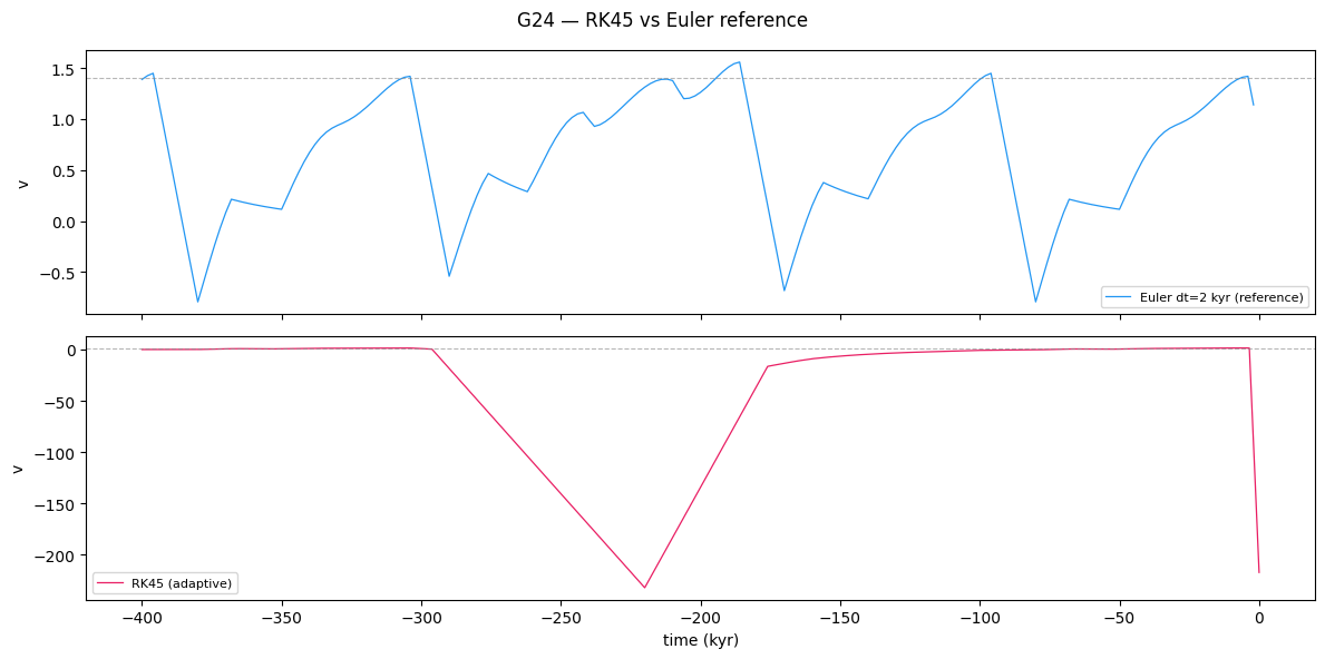

Note. RK45 either fails outright or produces a qualitatively wrong ice-volume record for G24. The root cause is that Model3 evaluates a threshold (v ≥ v_c and f ≥ f2) at every derivative call — but RK45 evaluates the derivative at several internal sub-step times per step. A threshold crossing that occurs between two full steps triggers mid-stage, leaving the model in the wrong regime for the remainder of the step. Fixed-step solvers (euler, rk4) evaluate the derivative exactly once per step, so threshold logic fires at the correct time.

SDEs: noise requires purpose-built integrators

When a model has stochastic forcing (set via model.sde_noise), the noise term must be handled by an SDE-aware method — euler_maruyama, heun_maruyama, or milstein. Passing a deterministic solver like RK45 silently ignores the noise entirely: RK45 evaluates the derivative at several internal sub-steps and never calls the noise function, so you get a deterministic trajectory that looks correct but contains none of the intended stochasticity.

sigma = 0.8   # noise amplitude (K yr^{-1/2})
def sde_noise_fn(t, state):
    return np.array([sigma])

N_ENS = 15
T_SPAN_SDE = (0, 500)
DT_SDE     = 1.0

# SDE ensemble with heun_maruyama (correct)
ens_sde = []
for seed in range(N_ENS):
    m = EBM0D(); m.sde_noise = sde_noise_fn
    out = m.integrate(t_span=T_SPAN_SDE, y0=[255.0], method='heun_maruyama',
                      kwargs={'dt': DT_SDE, 'random_seed': seed})
    ens_sde.append(out)

# RK45 with sde_noise set — noise is silently ignored
m_rk45_sde = EBM0D(); m_rk45_sde.sde_noise = sde_noise_fn
out_rk45_sde = m_rk45_sde.integrate(t_span=T_SPAN_SDE, y0=[255.0], method='RK45')

fig, axes = plt.subplots(1, 2, figsize=(13, 4), sharey=True)

# Left: heun_maruyama ensemble
for out in ens_sde:
    axes[0].plot(out.time, out.state_variables['T'],
                 color='steelblue', lw=0.6, alpha=0.35)
axes[0].plot(ens_sde[0].time,
             np.mean([o.state_variables['T'] for o in ens_sde], axis=0),
             color='navy', lw=2, label='ensemble mean')
axes[0].set_title('heun_maruyama  (correct SDE solver)')
axes[0].set_xlabel('time (yr)'); axes[0].set_ylabel('T (K)')
axes[0].legend(fontsize=8)

# Right: RK45 — flat deterministic line despite sde_noise being set
axes[1].plot(out_rk45_sde.time, out_rk45_sde.state_variables['T'],
             color='firebrick', lw=1.5, label='RK45 (sde_noise ignored)')
axes[1].set_title('RK45 with sde_noise set  (noise silently ignored)')
axes[1].set_xlabel('time (yr)')
axes[1].legend(fontsize=8)

fig.suptitle('EBM0D — SDE solver vs deterministic solver with noise term set')
plt.tight_layout(); plt.show()

<positron-console-cell-11>:13: DeprecationWarning: Passing 'dt' inside kwargs is deprecated and will be removed in a future version. Use the explicit parameter: integrate(..., dt=value).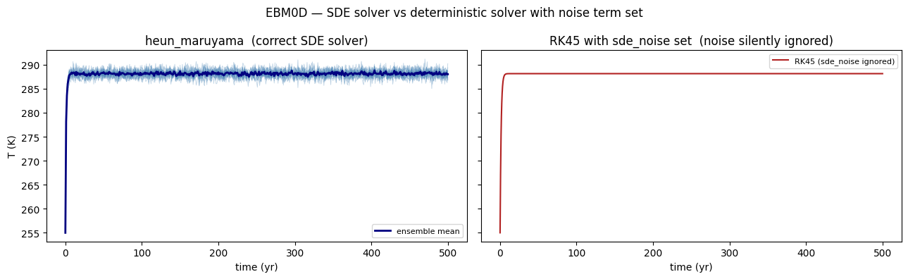

Figure. Left: heun_maruyama produces a spread of stochastic realisations around the deterministic transient — the noise is correctly integrated at each step. Right: RK45 with the same sde_noise function set returns a single smooth trajectory identical to the noiseless run; the noise function is never called. Use euler_maruyama, heun_maruyama, or milstein whenever model.sde_noise is set.

Lorenz96: stiff fast-slow system

The two-scale Lorenz96 model (J > 0) couples slow atmospheric variables \(X_k\) to \(J\) fast variables \(Y_{k,j}\). The fast variables evolve on timescales ~10× shorter than the slow ones, making the system mildly stiff.

Adaptive solvers fail here. Scipy’s RK45 evaluates dydt at sub-step quadrature points to estimate local error. For a model that accumulates state history during dydt (as L96 does for its Y-variable bookkeeping), those sub-step evaluations corrupt the history array and produce a trajectory that is physically wrong — not just inaccurate, but completely different from the true solution.

Use method='rk4' with an explicit fixed dt ≤ 0.005.

This example also appears in the lorenz96 model demo, where it is presented in the context of the full model walkthrough. It is reproduced here for thematic completeness.

K, J_val = 36, 10
F_ts     = 10.0
rng      = np.random.default_rng(42)

y0 = np.concatenate([rng.standard_normal(K) + F_ts,
                     rng.standard_normal(K * J_val) * 0.01])

# Correct: rk4 with explicit dt and si
model_rk4 = Lorenz96(n=K, F=F_ts, J=J_val, h=1.0, b=10.0, c=10.0)
out_rk4   = model_rk4.integrate(
    t_span=(0, 10), y0=y0.tolist(), method='rk4',
    dt=0.005, kwargs={'si': 0.005}
)

# Wrong: RK45 adaptive — sub-step evaluations corrupt Y history
try:
    model_rk45 = Lorenz96(n=K, F=F_ts, J=J_val, h=1.0, b=10.0, c=10.0)
    out_rk45   = model_rk45.integrate(
        t_span=(0, 10), y0=y0.tolist(), method='RK45', kwargs={}
    )
    rk45_ok = True
except Exception as e:
    print(f'RK45 raised: {e}')
    rk45_ok = False

X_rk4 = np.array([out_rk4.state_variables[f'x{k}'] for k in range(K)])
t_rk4 = out_rk4.time

# gridspec: two equal plot columns + a narrow dedicated colorbar column
fig = plt.figure(figsize=(13, 4))
gs  = fig.add_gridspec(1, 1 + rk45_ok, width_ratios=[1, 1], wspace=0.2)




# fig, axes = plt.subplots(1 + rk45_ok, 1, figsize=(12, 5 if not rk45_ok else 8),
#                          sharex=True if rk45_ok else False)

if not rk45_ok:
    gs = [gs]
    
gs0 = gs[0].subgridspec(1, 2, width_ratios = [1,.03],wspace=0.05 )
ax0 = fig.add_subplot(gs0[0])
cax0 = fig.add_subplot(gs0[1])

im0 = ax0.imshow(X_rk4.T, aspect='auto', origin='lower',
                     extent=[t_rk4[0], t_rk4[-1], -0.5, K - 0.5],
                     cmap='RdBu_r', vmin=-15, vmax=15)
plt.colorbar(im0, cax=cax0)
ax0.set(ylabel='site k', title='rk4 (dt=0.005) — correct', xlabel='time')

if rk45_ok:
    gs1 = gs[1].subgridspec(1, 2, width_ratios = [1,.03],wspace=0.05 )
    ax1 = fig.add_subplot(gs1[0])
    cax1 = fig.add_subplot(gs1[1])
    X_rk45 = np.array([out_rk45.state_variables[f'x{k}'] for k in range(K)])
    t_rk45 = out_rk45.time
    im1 = ax1.imshow(X_rk45.T, aspect='auto', origin='lower',
                         extent=[t_rk45[0], t_rk45[-1], -0.5, K - 0.5],
                         cmap='RdBu_r', vmin=-15, vmax=15)
    plt.colorbar(im1, cax=cax1)
    ax1.set(ylabel='site k', title='RK45 (adaptive) — corrupted history', xlabel='time', ylim=ax0.get_ylim())

fig.suptitle('Lorenz96 two-scale: rk4 vs RK45')
plt.tight_layout(); plt.show()

<positron-console-cell-13>:40: UserWarning: This figure includes Axes that are not compatible with tight_layout, so results might be incorrect.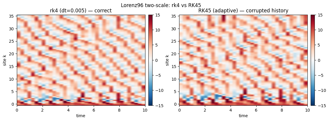

Figure. Space-time diagram of slow variable \(X_k\) for the two-scale system. The rk4 run (top) shows the correct pattern: eastward-propagating wave packets breaking into chaotic bursts, identical to the single-scale system at qualitative level. If RK45 does not crash (whether it crashes depends on the implementation version), its output shows either explosive growth or spurious spatial patterns — artefacts of corrupted sub-step Y-variable history. Even when the error is silent, the trajectory diverges from truth within a few time units.

Summary: solver selection guide

Model class	Recommended	Avoid	Key constraint
Smooth ODE (EBM0D, Stommel, ENSORecharge, Rössler, Lorenz63)	`RK45` (default)	`euler` unless timestep-matched	Use CC tight tolerances
Discrete-event ODE (G24)	`euler`, dt ≤ 6.5 kyr	`RK45`, `heun_maruyama`	Threshold crossings mis-stepped by adaptive solvers
Single-scale Lorenz96	`RK45` or `rk4`	—	`dt=0.05` adequate for space-time diagnostics
Two-scale Lorenz96	`rk4`, dt ≤ 0.005	`RK45` (corrupts Y history)	`si` (recording interval) set equal to `dt`
DampedSpring / SimplePendulum	`RK45`	`euler`	Stiff regimes need tight rtol
DoublePendulum (energy diagnostics)	`RK45` with rtol ≤ 1e-8	Default tolerances	Energy error scales with rtol
SDE models	`euler_maruyama`, `heun_maruyama`, or `milstein`	`RK45`	Must supply `sde_noise`; pass `random_seed` for reproducibility